Introduction to clustifyr
Rui Fu
RNA Bioscience Initative, University of Colorado School of MedicineAustin Gillen
RNA Bioscience Initative, University of Colorado School of MedicineRyan Sheridan
RNA Bioscience Initative, University of Colorado School of MedicineChengzhe Tian
Department of Biochemistry, University of Colorado BoulderMichelle Daya
Biomedical Informatics & Personalized Medicine, University of Colorado Anschutz Medical CampusYue Hao
Bioinformatics Research Center, North Carolina State UniversityJay Hesselberth
RNA Bioscience Initative, University of Colorado School of MedicineKent Riemondy
RNA Bioscience Initative, University of Colorado School of Medicine2025-04-16
Source:vignettes/clustifyr.Rmd
clustifyr.RmdIntroduction: Why use clustifyr?
Single cell transcriptomes are difficult to annotate without extensive knowledge of the underlying biology of the system in question. Even with this knowledge, accurate identification can be challenging due to the lack of detectable expression of common marker genes defined by bulk RNA-seq, flow cytometry, other single cell RNA-seq platforms, etc.
clustifyr solves this problem by providing functions to
automatically annotate single cells or clusters using bulk RNA-seq data
or marker gene lists (ranked or unranked). Additional functions allow
for exploratory analysis of calculated similarities between single cell
RNA-seq datasets and reference data.
Installation
To install clustifyr BiocManager must be installed.
install.packages("BiocManager")

BiocManager::install("clustifyr")
A simple example: 10x Genomics PBMCs
In this example, we take a 10x Genomics 3’ scRNA-seq dataset from
peripheral blood mononuclear cells (PBMCs) and annotate the cell
clusters (identified using Seurat) using scRNA-seq cell
clusters assigned from a CITE-seq experiment.
library(clustifyr)
library(ggplot2)
library(cowplot)

# Matrix of normalized single-cell RNA-seq counts
pbmc_matrix <- clustifyr::pbmc_matrix_small

# meta.data table containing cluster assignments for each cell
# The table that we are using also contains the known cell identities in the "classified" column
pbmc_meta <- clustifyr::pbmc_meta
Calculate correlation coefficients
To identify cell types, the clustifyr() function
requires several inputs:
-
input: an SingleCellExperiment or Seurat object or a matrix of normalized single-cell RNA-seq counts -
metadata: a meta.data table containing the cluster assignments for each cell (not required if a Seurat object is given) -
ref_mat: a reference matrix containing RNA-seq expression data for each cell type of interest -
query_genes: a list of genes to use for comparison (optional but recommended)
When using a matrix of scRNA-seq counts clustifyr() will
return a matrix of correlation coefficients for each cell type and
cluster, with the rownames corresponding to the cluster number.
# Calculate correlation coefficients for each cluster (spearman by default)
vargenes <- pbmc_vargenes[1:500]

res <- clustify(
    input = pbmc_matrix, # matrix of normalized scRNA-seq counts (or SCE/Seurat object)
    metadata = pbmc_meta, # meta.data table containing cell clusters
    cluster_col = "seurat_clusters", # name of column in meta.data containing cell clusters
    ref_mat = cbmc_ref, # matrix of RNA-seq expression data for each cell type
    query_genes = vargenes # list of highly varible genes identified with Seurat
)

# Peek at correlation matrix
res[1:5, 1:5]
#>           B CD14+ Mono CD16+ Mono     CD34+     CD4 T
#> 0 0.6563466  0.6454029  0.6485863 0.7089861 0.8804508
#> 1 0.6394363  0.6388404  0.6569401 0.7027430 0.8488750
#> 2 0.5524081  0.9372089  0.8930158 0.5879264 0.5347312
#> 3 0.8945380  0.5801453  0.6146857 0.6955897 0.6566739
#> 4 0.5711643  0.5623870  0.5826233 0.6280913 0.7467347

# Call cell types
res2 <- cor_to_call(
    cor_mat = res, # matrix correlation coefficients
    cluster_col = "seurat_clusters" # name of column in meta.data containing cell clusters
)
res2[1:5, ]
#> # A tibble: 5 × 3
#> # Groups:   seurat_clusters [5]
#>   seurat_clusters type           r
#>   <chr>           <chr>      <dbl>
#> 1 3               B          0.895
#> 2 2               CD14+ Mono 0.937
#> 3 5               CD16+ Mono 0.929
#> 4 0               CD4 T      0.880
#> 5 1               CD4 T      0.849

# Insert into original metadata as "type" column
pbmc_meta2 <- call_to_metadata(
    res = res2, # data.frame of called cell type for each cluster
    metadata = pbmc_meta, # original meta.data table containing cell clusters
    cluster_col = "seurat_clusters" # name of column in meta.data containing cell clusters
)
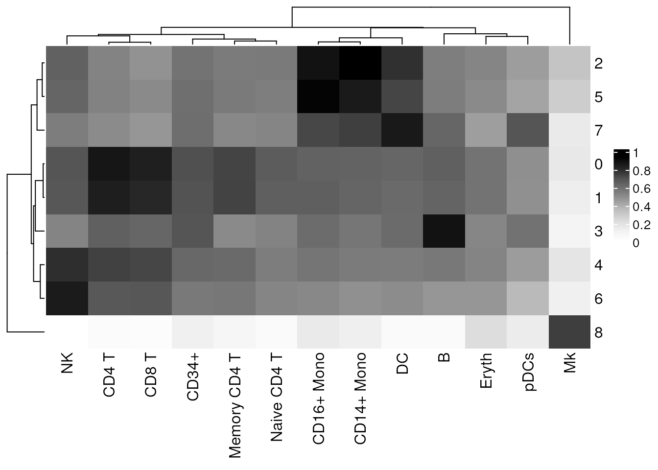
To visualize the clustifyr() results we can use the
plot_cor_heatmap() function to plot the correlation
coefficients for each cluster and each cell type.
# Create heatmap of correlation coefficients using clustifyr() output
plot_cor_heatmap(cor_mat = res)
Plot cluster identities and correlation coefficients
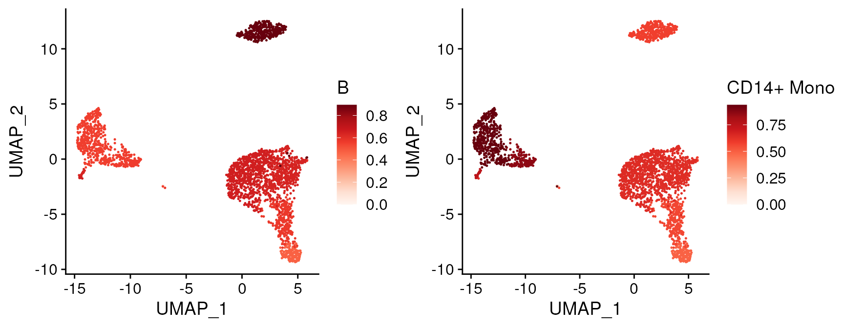
clustifyr also provides functions to overlay correlation
coefficients on pre-calculated tSNE embeddings (or those from any other
dimensionality reduction method).
# Overlay correlation coefficients on UMAPs for the first two cell types
corr_umaps <- plot_cor(
    cor_mat = res, # matrix of correlation coefficients from clustifyr()
    metadata = pbmc_meta, # meta.data table containing UMAP or tSNE data
    data_to_plot = colnames(res)[1:2], # name of cell type(s) to plot correlation coefficients
    cluster_col = "seurat_clusters" # name of column in meta.data containing cell clusters
)

plot_grid(
    plotlist = corr_umaps,
    rel_widths = c(0.47, 0.53)
)
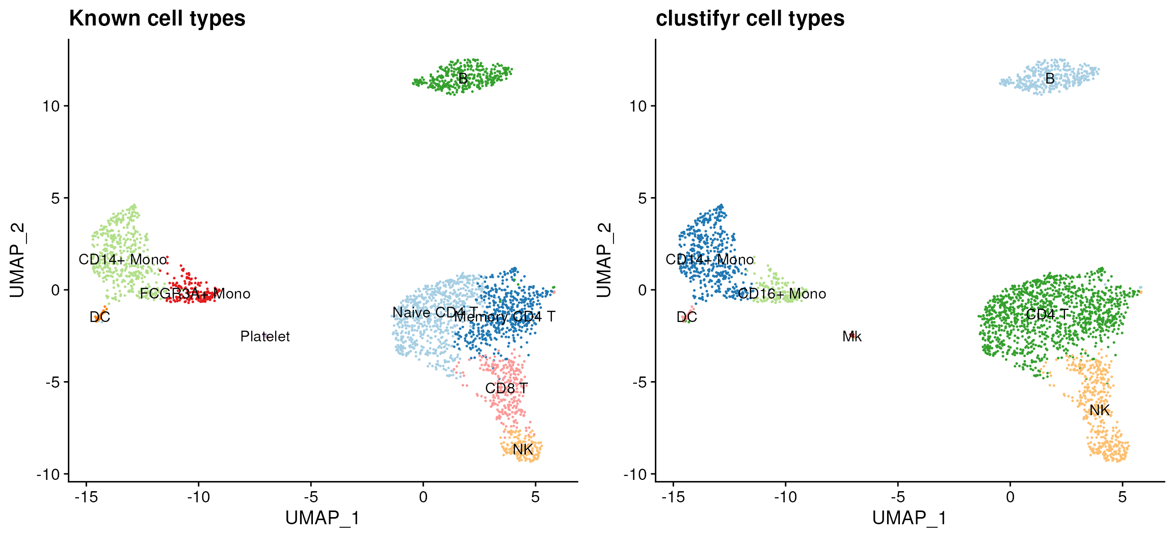
The plot_best_call() function can be used to label each
cluster with the cell type that gives the highest corelation
coefficient. Using the plot_dims() function, we can also
plot the known identities of each cluster, which were stored in the
“classified” column of the meta.data table. The plots below show that
the highest correlations between the reference RNA-seq data and the 10x
Genomics scRNA-seq dataset are restricted to the correct cell
clusters.
# Label clusters with clustifyr cell identities
clustifyr_types <- plot_best_call(
    cor_mat = res, # matrix of correlation coefficients from clustifyr()
    metadata = pbmc_meta, # meta.data table containing UMAP or tSNE data
    do_label = TRUE, # should the feature label be shown on each cluster?
    do_legend = FALSE, # should the legend be shown?
    do_repel = FALSE, # use ggrepel to avoid overlapping labels
    cluster_col = "seurat_clusters"
) +
    ggtitle("clustifyr cell types")

# Compare clustifyr results with known cell identities
known_types <- plot_dims(
    data = pbmc_meta, # meta.data table containing UMAP or tSNE data
    feature = "classified", # name of column in meta.data to color clusters by
    do_label = TRUE, # should the feature label be shown on each cluster?
    do_legend = FALSE, # should the legend be shown?
    do_repel = FALSE
) +
    ggtitle("Known cell types")

plot_grid(known_types, clustifyr_types)
Classify cells using known marker genes
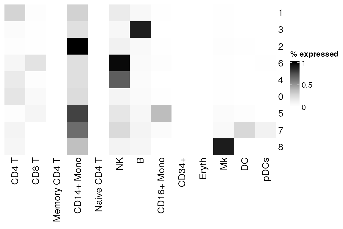
The clustify_lists() function allows cell types to be
assigned based on known marker genes. This function requires a table
containing markers for each cell type of interest. Cell types can be
assigned using several statistical tests including, hypergeometric,
Jaccard, Spearman, and GSEA.
# Take a peek at marker gene table
cbmc_m
#>   CD4 T CD8 T Memory CD4 T CD14+ Mono Naive CD4 T   NK     B CD16+ Mono
#> 1 ITM2A  CD8B        ADCY2     S100A8       CDHR3 GNLY  IGHM     CDKN1C
#> 2 TXNIP  CD8A       PTGDR2     S100A9  DICER1-AS1 NKG7 CD79A       HES4
#> 3   AES S100B      CD200R1        LYZ       RAD9A CST7 MS4A1        CKB
#>      CD34+ Eryth    Mk    DC   pDCs
#> 1   SPINK2   HBM   PF4  ENHO LILRA4
#> 2  C1QTNF4  AHSP  SDPR  CD1E   TPM2
#> 3 KIAA0125   CA1 TUBB1 NDRG2    SCT

# Available metrics include: "hyper", "jaccard", "spearman", "gsea"
list_res <- clustify_lists(
    input = pbmc_matrix, # matrix of normalized single-cell RNA-seq counts
    metadata = pbmc_meta, # meta.data table containing cell clusters
    cluster_col = "seurat_clusters", # name of column in meta.data containing cell clusters
    marker = cbmc_m, # list of known marker genes
    metric = "pct" # test to use for assigning cell types
)

# View as heatmap, or plot_best_call
plot_cor_heatmap(
    cor_mat = list_res, # matrix of correlation coefficients from clustify_lists()
    cluster_rows = FALSE, # cluster by row?
    cluster_columns = FALSE, # cluster by column?
    legend_title = "% expressed" # title of heatmap legend
)
# Downstream functions same as clustify()
# Call cell types
list_res2 <- cor_to_call(
    cor_mat = list_res, # matrix correlation coefficients
    cluster_col = "seurat_clusters" # name of column in meta.data containing cell clusters
)

# Insert into original metadata as "list_type" column
pbmc_meta3 <- call_to_metadata(
    res = list_res2, # data.frame of called cell type for each cluster
    metadata = pbmc_meta, # original meta.data table containing cell clusters
    cluster_col = "seurat_clusters", # name of column in meta.data containing cell clusters
    rename_prefix = "list_" # set a prefix for the new column
)
Direct handling of SingleCellExperiment objects
clustifyr can also use a
SingleCellExperiment object as input and return a new
SingleCellExperiment object with the cell types added as a
column in the colData.
library(SingleCellExperiment)
sce <- sce_pbmc()
res <- clustify(
    input = sce, # an SCE object
    ref_mat = cbmc_ref, # matrix of RNA-seq expression data for each cell type
    cluster_col = "clusters", # name of column in meta.data containing cell clusters
    obj_out = TRUE # output SCE object with cell type inserted as "type" column
)

colData(res)[1:10, c("type", "r")]
#> DataFrame with 10 rows and 2 columns
#>                       type         r
#>                <character> <numeric>
#> AAACATACAACCAC       CD4 T  0.861083
#> AAACATTGAGCTAC           B  0.909358
#> AAACATTGATCAGC       CD4 T  0.861083
#> AAACCGTGCTTCCG  CD14+ Mono  0.914543
#> AAACCGTGTATGCG          NK  0.894090
#> AAACGCACTGGTAC       CD4 T  0.861083
#> AAACGCTGACCAGT          NK  0.825784
#> AAACGCTGGTTCTT          NK  0.825784
#> AAACGCTGTAGCCA       CD4 T  0.889149
#> AAACGCTGTTTCTG  CD16+ Mono  0.929491
Direct handling of Seurat objects
clustifyr can also use a Seurat object as
input and return a new Seurat object with the cell types
added as a column in the meta.data.
so <- so_pbmc()
res <- clustify(
    input = so, # a Seurat object
    ref_mat = cbmc_ref, # matrix of RNA-seq expression data for each cell type
    cluster_col = "seurat_clusters", # name of column in meta.data containing cell clusters
    obj_out = TRUE # output Seurat object with cell type inserted as "type" column
)

# type and r are stored in the meta.data
res[[c("type", "r")]][1:10, ]
#>                      type         r
#> AAACATACAACCAC      CD4 T 0.8424452
#> AAACATTGAGCTAC          B 0.8984684
#> AAACATTGATCAGC      CD4 T 0.8424452
#> AAACCGTGCTTCCG CD14+ Mono 0.9319558
#> AAACCGTGTATGCG         NK 0.8816119
#> AAACGCACTGGTAC      CD4 T 0.8424452
#> AAACGCTGACCAGT         NK 0.8147040
#> AAACGCTGGTTCTT         NK 0.8147040
#> AAACGCTGTAGCCA      CD4 T 0.8736163
#> AAACGCTGTTTCTG CD16+ Mono 0.9321784
Building reference matrix from single cell expression matrix
In its simplest form, a reference matrix is built by averaging expression (also includes an option to take the median) of a single cell RNA-seq expression matrix by cluster. Both log transformed or raw count matrices are supported.
new_ref_matrix <- average_clusters(
    mat = pbmc_matrix,
    metadata = pbmc_meta$classified, # or use metadata = pbmc_meta, cluster_col = "classified"
    if_log = TRUE # whether the expression matrix is already log transformed
)

head(new_ref_matrix)
#>                 B CD14+ Mono      CD8 T         DC FCGR3A+ Mono Memory CD4 T
#> PPBP   0.09375021 0.28763857 0.35662599 0.06527347    0.2442300   0.06494743
#> LYZ    1.42699419 5.21550849 1.35146753 4.84714962    3.4034309   1.39466552
#> S100A9 0.62123058 4.91453355 0.58823794 2.53310734    2.6277996   0.58080250
#> IGLL5  2.44576997 0.02434753 0.03284986 0.10986617    0.2581198   0.04826212
#> GNLY   0.37877736 0.53592906 2.53161887 0.46959958    0.2903092   0.41001072
#> FTL    3.66698837 5.86217774 3.37056910 4.21848878    5.9518479   3.31062958
#>        Naive CD4 T         NK  Platelet
#> PPBP    0.04883837 0.00000000 6.0941782
#> LYZ     1.40165143 1.32701580 2.5303912
#> S100A9  0.55679700 0.52098541 1.6775692
#> IGLL5   0.03116080 0.05247669 0.2501642
#> GNLY    0.46041901 4.70481754 0.3845813
#> FTL     3.35611600 3.38471536 4.5508242

# For further convenience, a shortcut function for generating reference matrix from `SingleCellExperiment` or `seurat` object is used.
new_ref_matrix_sce <- object_ref(
    input = sce, # SCE object
    cluster_col = "clusters" # name of column in colData containing cell identities
)

new_ref_matrix_so <- seurat_ref(
    seurat_object = so, # Seurat object
    cluster_col = "seurat_clusters" # name of column in meta.data containing cell identities
)

tail(new_ref_matrix_so)
#>                  0          1           2          3          4          5
#> RHOC   0.245754269 0.40431050 0.590053057 0.37702525 0.86466156 2.20162898
#> CISH   0.492444272 0.54773003 0.079843557 0.08962348 0.66024943 0.10588034
#> CD27   1.195370020 1.28719850 0.100562312 0.54487892 1.28322681 0.09640885
#> LILRA3 0.004576215 0.03686387 0.544743180 0.00000000 0.03409087 1.35418074
#> CLIC2  0.007570624 0.00000000 0.021200958 0.00000000 0.00000000 0.00000000
#> HEMGN  0.034099324 0.04619359 0.006467157 0.00000000 0.00000000 0.00000000
#>                6          7        8
#> RHOC   1.6518448 0.72661911 1.465067
#> CISH   0.1339815 0.18231747 0.000000
#> CD27   0.1600911 0.04639912 0.000000
#> LILRA3 0.0000000 0.00000000 0.000000
#> CLIC2  0.0000000 0.46542832 0.000000
#> HEMGN  0.0000000 0.00000000 1.079083
More reference data, including tabula muris, and code used to generate them are available at https://github.com/rnabioco/clustifyrdata
Also see list for individual downloads at https://rnabioco.github.io/clustifyrdata/articles/download_refs.html
Additional tutorials at https://rnabioco.github.io/clustifyrdata/articles/otherformats.html
Session info
sessionInfo()
#> R version 4.4.2 (2024-10-31)
#> Platform: x86_64-pc-linux-gnu
#> Running under: Ubuntu 24.04.1 LTS
#>
#> Matrix products: default
#> BLAS:   /usr/lib/x86_64-linux-gnu/openblas-pthread/libblas.so.3
#> LAPACK: /usr/lib/x86_64-linux-gnu/openblas-pthread/libopenblasp-r0.3.26.so;  LAPACK version 3.12.0
#>
#> locale:
#>  [1] LC_CTYPE=en_US.UTF-8       LC_NUMERIC=C
#>  [3] LC_TIME=en_US.UTF-8        LC_COLLATE=en_US.UTF-8
#>  [5] LC_MONETARY=en_US.UTF-8    LC_MESSAGES=en_US.UTF-8
#>  [7] LC_PAPER=en_US.UTF-8       LC_NAME=C
#>  [9] LC_ADDRESS=C               LC_TELEPHONE=C
#> [11] LC_MEASUREMENT=en_US.UTF-8 LC_IDENTIFICATION=C
#>
#> time zone: UTC
#> tzcode source: system (glibc)
#>
#> attached base packages:
#> [1] stats4    stats     graphics  grDevices utils     datasets  methods
#> [8] base
#>
#> other attached packages:
#>  [1] SingleCellExperiment_1.28.1 SummarizedExperiment_1.36.0
#>  [3] Biobase_2.66.0              GenomicRanges_1.58.0
#>  [5] GenomeInfoDb_1.42.3         IRanges_2.40.1
#>  [7] S4Vectors_0.44.0            BiocGenerics_0.52.0
#>  [9] MatrixGenerics_1.18.1       matrixStats_1.5.0
#> [11] cowplot_1.1.3               ggplot2_3.5.2
#> [13] clustifyr_1.21.0            BiocStyle_2.34.0
#>
#> loaded via a namespace (and not attached):
#>  [1] rlang_1.1.6             magrittr_2.0.3          clue_0.3-66
#>  [4] GetoptLong_1.0.5        compiler_4.4.2          png_0.1-8
#>  [7] systemfonts_1.2.2       vctrs_0.6.5             pkgconfig_2.0.3
#> [10] shape_1.4.6.1           crayon_1.5.3            fastmap_1.2.0
#> [13] XVector_0.46.0          labeling_0.4.3          utf8_1.2.4
#> [16] rmarkdown_2.29          UCSC.utils_1.2.0        ragg_1.4.0
#> [19] purrr_1.0.4             xfun_0.52               zlibbioc_1.52.0
#> [22] cachem_1.1.0            jsonlite_2.0.0          DelayedArray_0.32.0
#> [25] BiocParallel_1.40.2     parallel_4.4.2          cluster_2.1.8.1
#> [28] R6_2.6.1                bslib_0.9.0             RColorBrewer_1.1-3
#> [31] parallelly_1.43.0       jquerylib_0.1.4         Rcpp_1.0.14
#> [34] bookdown_0.43           iterators_1.0.14        knitr_1.50
#> [37] future.apply_1.11.3     Matrix_1.7-3            tidyselect_1.2.1
#> [40] abind_1.4-8             yaml_2.3.10             doParallel_1.0.17
#> [43] codetools_0.2-20        listenv_0.9.1           lattice_0.22-7
#> [46] tibble_3.2.1            withr_3.0.2             evaluate_1.0.3
#> [49] future_1.40.0           desc_1.4.3              circlize_0.4.16
#> [52] pillar_1.10.2           BiocManager_1.30.25     foreach_1.5.2
#> [55] generics_0.1.3          sp_2.2-0                munsell_0.5.1
#> [58] scales_1.3.0            globals_0.16.3          glue_1.8.0
#> [61] tools_4.4.2             data.table_1.17.0       fgsea_1.32.4
#> [64] fs_1.6.6                dotCall64_1.2           fastmatch_1.1-6
#> [67] grid_4.4.2              tidyr_1.3.1             colorspace_2.1-1
#> [70] GenomeInfoDbData_1.2.13 cli_3.6.4               textshaping_1.0.0
#> [73] spam_2.11-1             S4Arrays_1.6.0          ComplexHeatmap_2.22.0
#> [76] dplyr_1.1.4             gtable_0.3.6            sass_0.4.10
#> [79] digest_0.6.37           progressr_0.15.1        SparseArray_1.6.2
#> [82] farver_2.1.2            rjson_0.2.23            htmlwidgets_1.6.4
#> [85] SeuratObject_5.0.2      entropy_1.3.2           htmltools_0.5.8.1
#> [88] pkgdown_2.1.1           lifecycle_1.0.4         httr_1.4.7
#> [91] GlobalOptions_0.1.2