Plotting tSNE and UMAP results
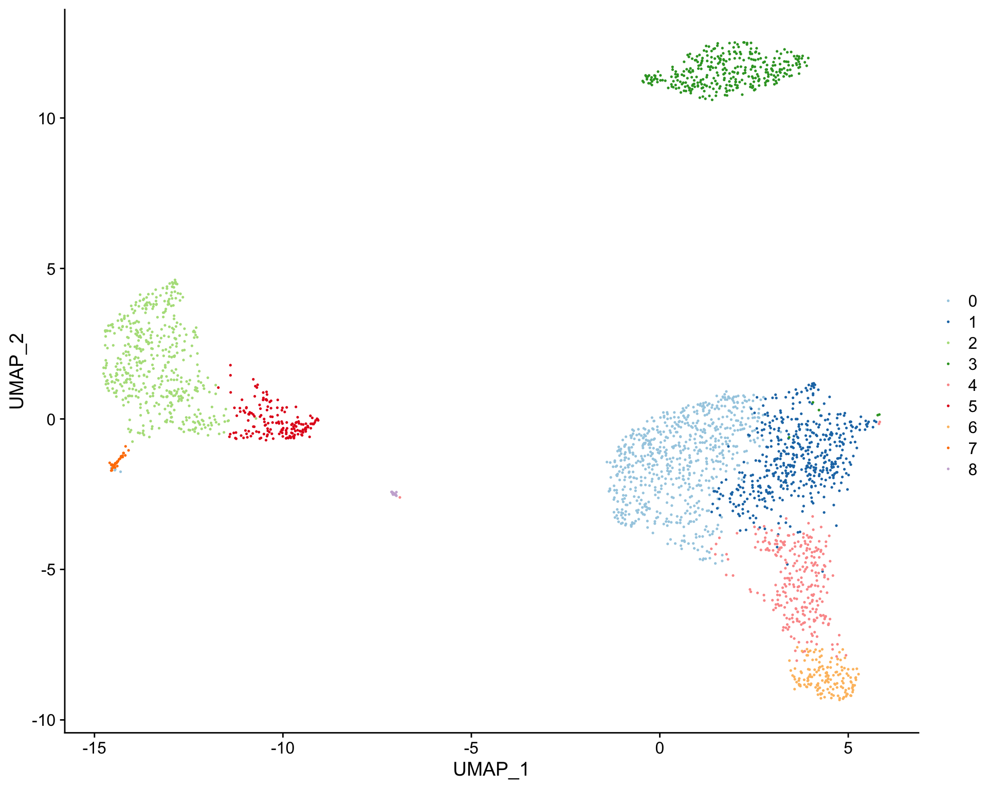
clustifyr provides several functions to plot tSNE or UMAP results. The plot_dims() function will plot tSNE or UMAP data using a meta.data table and can color the cells based on cluster identity.
library(clustifyr)
library(clustifyrdata)

library(dplyr)
library(tibble)

# Matrix of normalized single-cell RNA-seq counts
pbmc_matrix[1:3, 1:3]
#> 3 x 3 sparse Matrix of class "dgCMatrix"
#>               AAACATACAACCAC AAACATTGAGCTAC AAACATTGATCAGC
#> AL627309.1                 .              .              .
#> AP006222.2                 .              .              .
#> RP11-206L10.2              .              .              .

# meta.data table containing cluster assignments for each cell
pbmc_meta[1:5, ]
#>                orig.ident nCount_RNA nFeature_RNA percent.mt RNA_snn_res.0.5
#> AAACATACAACCAC     pbmc3k       2419          779  3.0177759               1
#> AAACATTGAGCTAC     pbmc3k       4903         1352  3.7935958               3
#> AAACATTGATCAGC     pbmc3k       3147         1129  0.8897363               1
#> AAACCGTGCTTCCG     pbmc3k       2639          960  1.7430845               2
#> AAACCGTGTATGCG     pbmc3k        980          521  1.2244898               6
#>                seurat_clusters   classified     UMAP_1     UMAP_2
#> AAACATACAACCAC               1 Memory CD4 T   2.341260 -3.0761487
#> AAACATTGAGCTAC               3            B   3.712070 11.7883301
#> AAACATTGATCAGC               1 Memory CD4 T   5.065264 -0.7839952
#> AAACCGTGCTTCCG               2   CD14+ Mono -11.783583  0.8343185
#> AAACCGTGTATGCG               6           NK   3.576498 -8.9778881

# Create tSNE and color cells based on cluster ID
plot_dims(
  x = "UMAP_1", # name of column in the meta.data containing the data to plot on x-axis
  y = "UMAP_2", # name of column in the meta.data containing the data to plot on y-axis
  data = pbmc_meta, # meta.data table containing cluster assignments for each cell
  feature = "seurat_clusters" # name of column in meta.data to color cells by
)
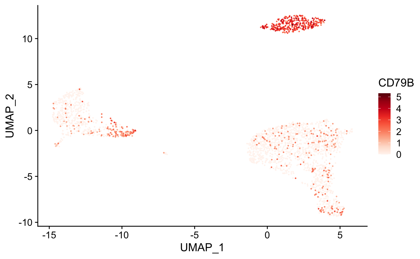
Cells can also be colored based on the expression level of a gene or list of genes using the plot_gene() function.
# Create tSNE and color cells based on gene expression
plot_gene(
  x = "UMAP_1", # name of column in the meta.data containing the data to plot on x-axis
  y = "UMAP_2", # name of column in the meta.data containing the data to plot on y-axis
  expr_mat = pbmc_matrix, # matrix of normalized single-cell RNA-seq counts
  metadata = pbmc_meta %>% rownames_to_column("rn"), # meta.data table containing cluster assignments for each cell
  genes = c("CD79B", "CD8A"), # vector of gene names to color cells
  cell_col = "rn" # name of column in meta.data containing the cell IDs
)
#> [[1]]
#>
#> [[2]]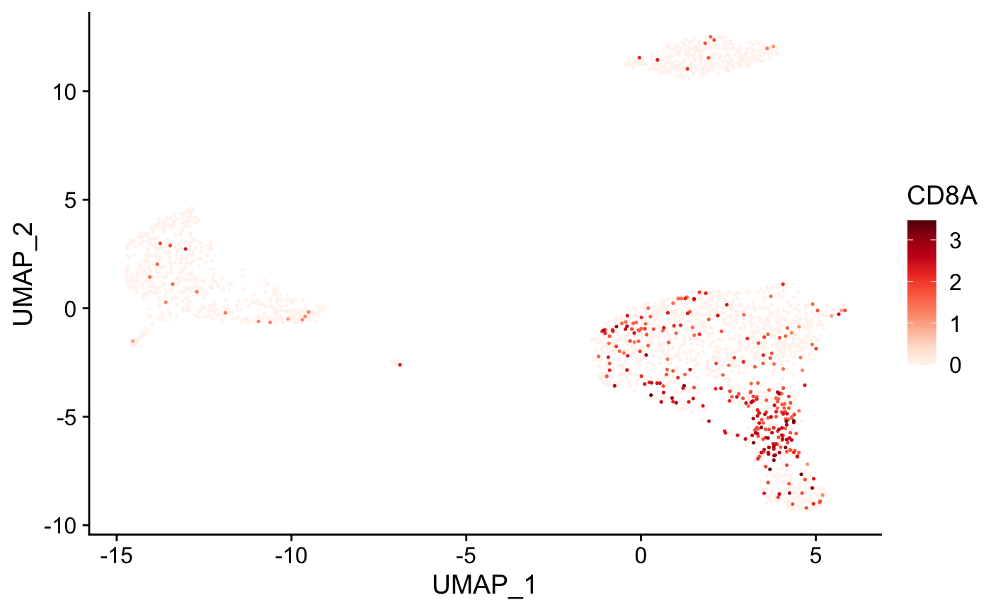
Visualizing clustifyr() results
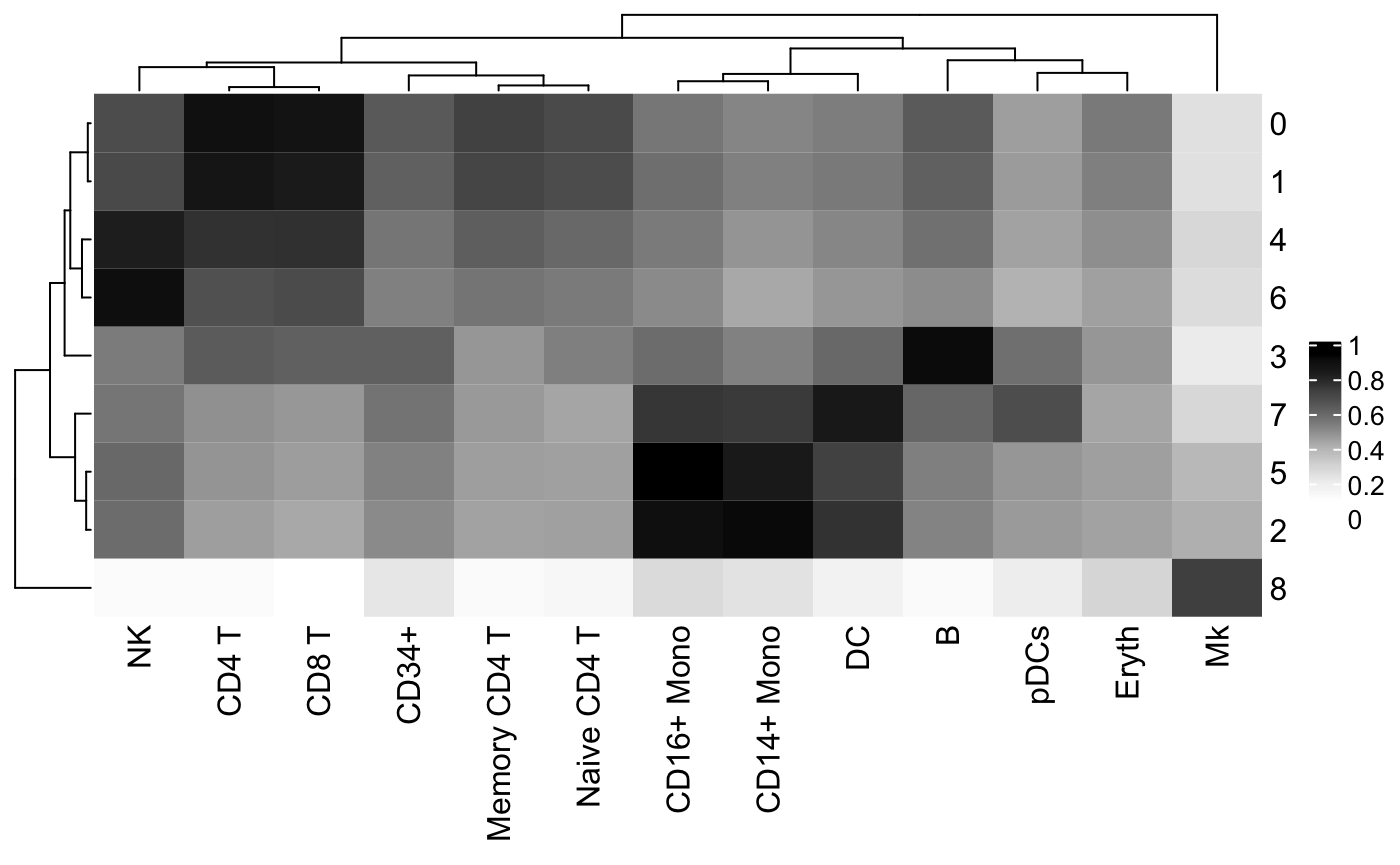
The clustifyr() function outputs a matrix of correlation coefficients and clustify_lists() and clustify_nudge() output positive scores. clustifyr provides built-in functions to help visualize these results.
Cell type assignments can be assessed by plotting the clustifyr() correlation matrix as a heatmap using the plot_cor_heatmap() function.
# Run clustifyr()
res <- clustify(
  input = pbmc_matrix, # matrix of normalized single-cell RNA-seq counts
  metadata = pbmc_meta, # meta.data table containing cluster assignments for each cell
  ref_mat = cbmc_ref, # reference matrix containing bulk RNA-seq data for each cell type
  query_genes = pbmc_vargenes, # list of highly varible genes identified with Seurat
  cluster_col = "seurat_clusters" # name of column in meta.data containing cell clusters
)
#> [1] "use"

# Create heatmap using the clustifyr correlation matrix
plot_cor_heatmap(
  cor_mat = res # matrix of correlation coefficients from clustifyr()
)
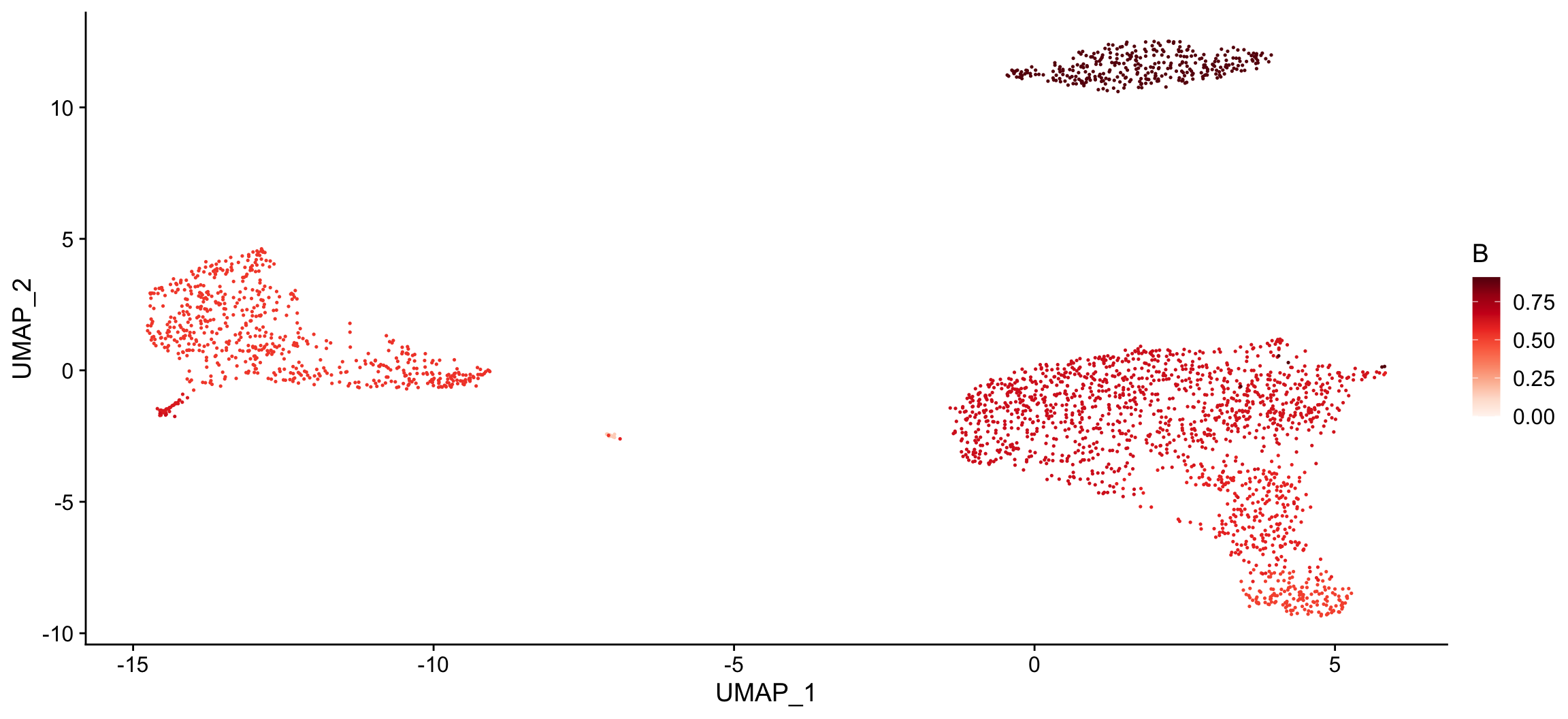
The plot_cor() function can also be used to create a tSNE for each cell type of interest and color the cells based on the correlation coefficients.
# Create a tSNE for each cell type of interest and color cells based on correlation coefficients
plot_cor(
  x = "UMAP_1", # name of column in the meta.data containing the data to plot on x-axis
  y = "UMAP_2", # name of column in the meta.data containing the data to plot on y-axis
  cor_mat = res, # matrix of correlation coefficients from clustifyr()
  metadata = pbmc_meta, # meta.data table containing cluster assignments for each cell
  data_to_plot = colnames(res)[1:2], # name of cell type(s) to plot correlation coefficients
  cluster_col = "seurat_clusters" # name of column in meta.data containing cell clusters
)
#> [[1]]
#>
#> [[2]]
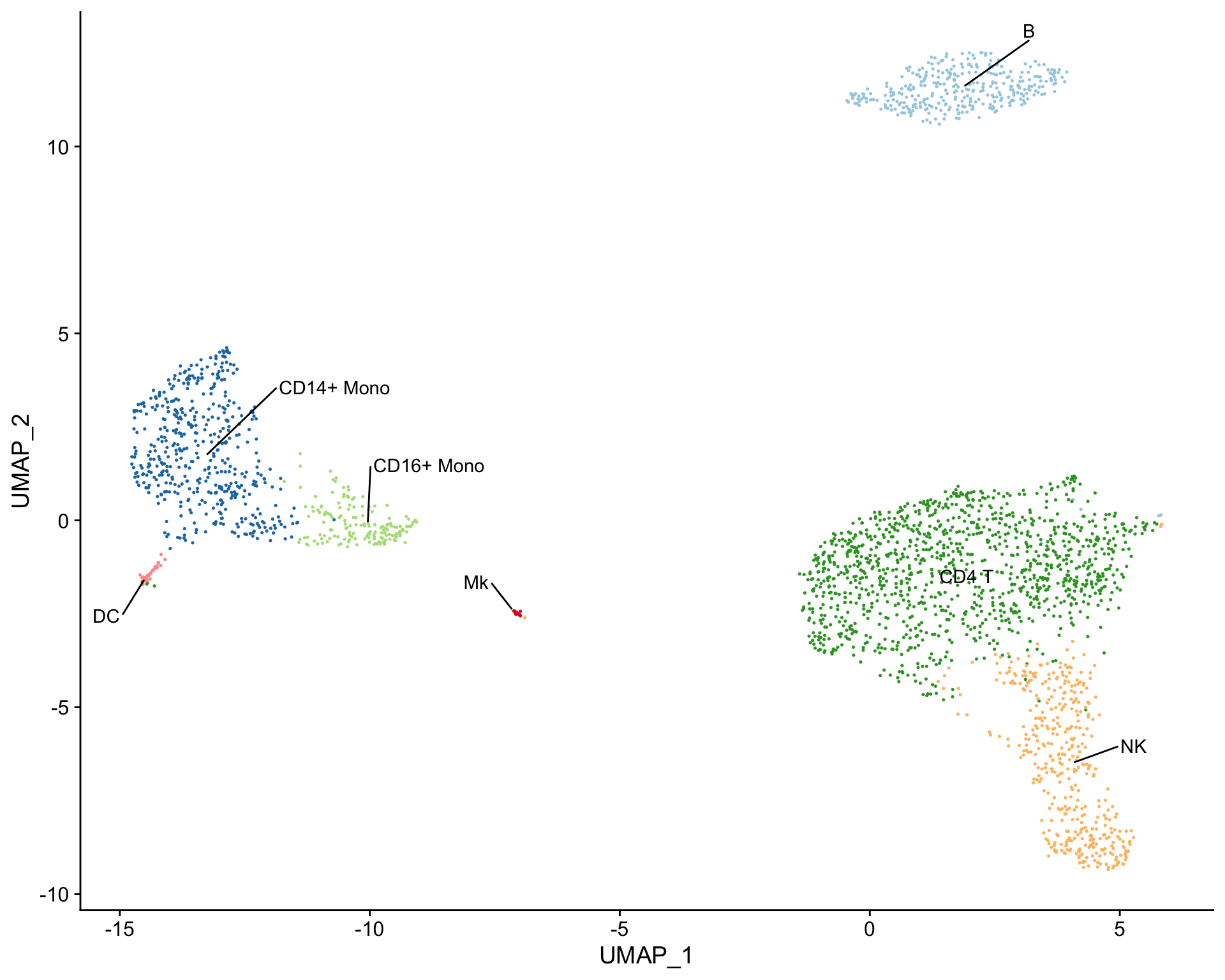
Cell clusters can also be labeled using the plot_best_call() function, which takes the correlation matrix and labels cell clusters with the cell type that has the highest correlation coefficient.
# Create tSNE and label clusters with the cell type that has the highest correlation coefficient
plot_best_call(
  cor_mat = res, # matrix of correlation coefficients from clustifyr()
  metadata = pbmc_meta, # meta.data table containing UMAP or tSNE data
  do_label = TRUE, # should the feature label be shown on each cluster?
  do_legend = FALSE, # should the legend be shown?
  cluster_col = "seurat_clusters"
)
Assessing clustifyr() accuracy
The clustifyr() results can also be evaluated by over-clustering the data and comparing the cell type assignments before and after over-clustering. This is accomplished using the overcluster_test() function. The cell type assignments should be similar with and without over-clustering.
# Overcluster cells and compare cell type assignments with and without over-clustering
overcluster_test(
  expr = pbmc_matrix, # matrix of normalized single-cell RNA-seq counts
  metadata = pbmc_meta, # meta.data table containing UMAP or tSNE data
  ref_mat = cbmc_ref, # reference matrix containing bulk RNA-seq data for each cell type
  cluster_col = "seurat_clusters", # name of column in meta.data containing cell clusters
  n = 5 # expand cluster number n-fold for overclustering
)
#> [1] "use"
#> [1] "use"
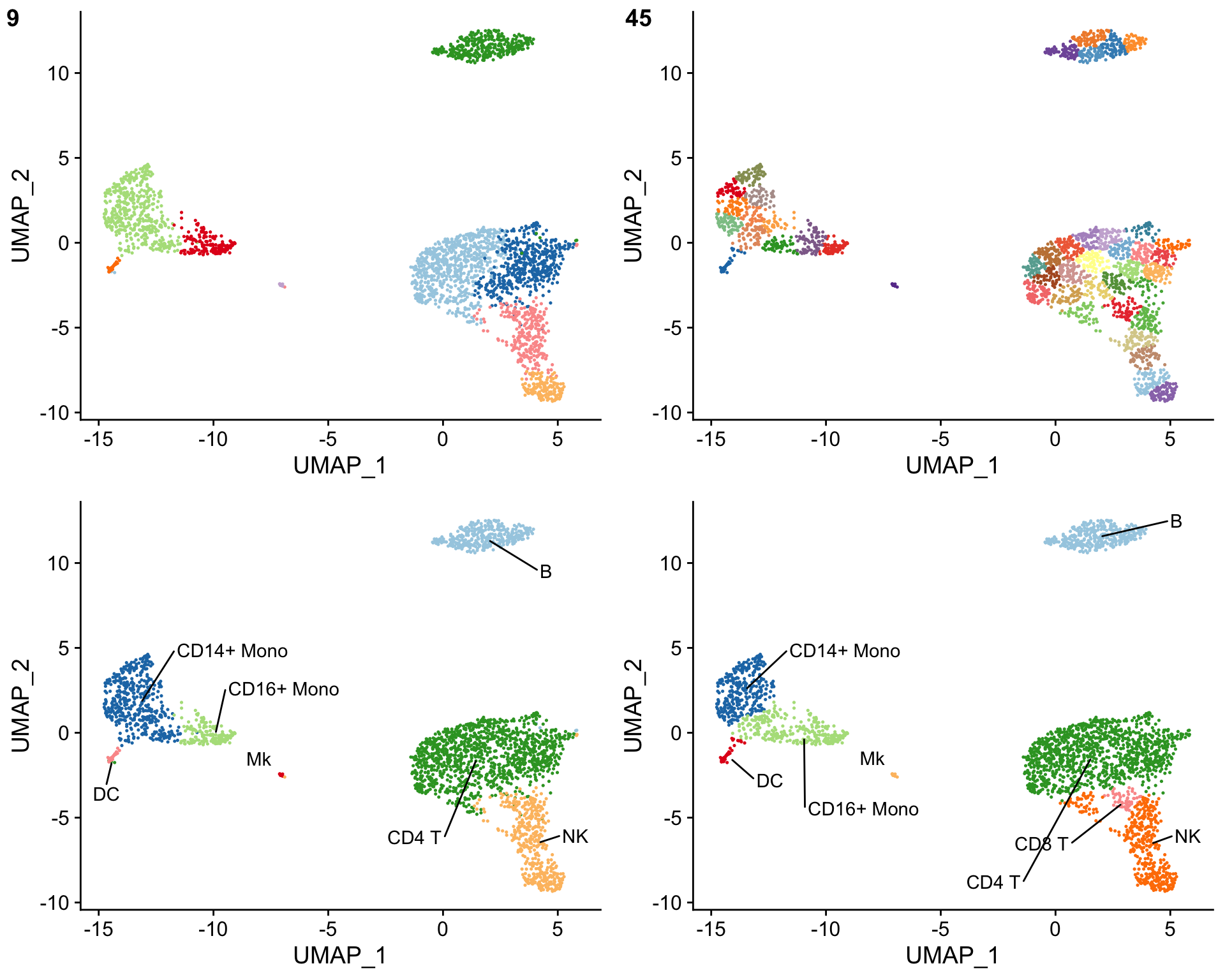
The cell types from the bulk RNA-seq reference matrix can also be mixed together using the make_comb_ref() function to assess the specificity of the cell type assignments. If a cluster shows a higher correlation when using the mixed reference matrix, this suggests that the cluster contains multiple cell types.
# Create reference containing different combinations of the bulk RNA-seq data
comb_ref <- make_comb_ref(
  ref_mat = cbmc_ref # reference matrix containing bulk RNA-seq data for each cell type
)

# Peek at the new combined reference
comb_ref[1:5, 1:5]

# Run clustifyr() using the combined reference
comb_res <- clustify(
  input = pbmc_matrix, # matrix of normalized single-cell RNA-seq counts
  metadata = pbmc_meta, # meta.data table containing cluster assignments for each cell
  ref_mat = comb_ref, # reference matrix containing bulk RNA-seq data for each cell type
  query_genes = pbmc_vargenes, # list of highly varible genes identified with Seurat
  cluster_col = "seurat_clusters" # name of column in meta.data containing cell clusters
)

# Create tSNE and label clusters with the assigned cell types from the combined reference
plot_best_call(
  cor_mat = comb_res, # matrix of correlation coefficients from clustifyr()
  metadata = pbmc_meta, # meta.data table containing UMAP or tSNE data
  do_label = TRUE, # should the feature label be shown on each cluster?
  do_legend = FALSE, # should the legend be shown?
  cluster_col = "seurat_clusters"
)
Plotting other attributes from the meta.data table
Visualization of other attributes shared in the metadata between ref and query by plot_cols, such as nGene, nUMI, mt_percentage, as another way of identity confirmation after clustify. Certain cell types have distinct patterns, more genes detected, for example.