Overview
This vignette demonstrates clover’s analysis workflow using E.
coli tRNA sequencing data from a T4 phage infection time-course
experiment. The test dataset includes 6 samples: 3 uninfected controls
(ctl) and 3 T4-infected (inf) wild-type E.
coli at 15 minutes post-infection, with 3 biological replicates per
condition.
Loading data with create_clover()
The simplest way to load results from the aa-tRNA-seq-pipeline
is with create_clover(), which reads a pipeline
configuration file and assembles a
SummarizedExperiment.
config_path <- clover_example("ecoli/config.yaml")

sample_info <- data.frame(
  sample_id = c(
    "wt-15-ctl-01",
    "wt-15-ctl-02",
    "wt-15-ctl-03",
    "wt-15-inf-01",
    "wt-15-inf-02",
    "wt-15-inf-03"
  ),
  condition = rep(c("ctl", "inf"), each = 3),
  replicate = rep(1:3, 2)
)

se <- create_clover(
  config_path,
  types = c("charging", "bcerror", "odds_ratios"),
  sample_info = sample_info
)

se
#> class: SummarizedExperiment
#> dim: 190 6
#> metadata(5): config charging bcerror odds_ratios fasta
#> assays(1): counts
#> rownames(190): host-tRNA-Ala-GGC-1-1 host-tRNA-Ala-GGC-1-1-uncharged
#>   ... phage-tRNA-Thr-TGT phage-tRNA-Thr-TGT-uncharged
#> rowData names(2): ref seq_length
#> colnames(6): wt-15-ctl-01 wt-15-ctl-02 ... wt-15-inf-02 wt-15-inf-03
#> colData names(3): sample_id condition replicate
The SE object contains:
- assay “counts”: abundance count matrix (charged + uncharged reads)
- colData: sample metadata with condition labels
- metadata: list with raw charging data, bcerror, odds ratios, FASTA reference, and pipeline config
assay(se, "counts")[1:5, ]
#>                                 wt-15-ctl-01 wt-15-ctl-02 wt-15-ctl-03
#> host-tRNA-Ala-GGC-1-1                    298          397          113
#> host-tRNA-Ala-GGC-1-1-uncharged         4393         5014          883
#> host-tRNA-Ala-GGC-1-2                   1625         1506          265
#> host-tRNA-Ala-GGC-1-2-uncharged         4391         5130          862
#> host-tRNA-Ala-TGC-1-1                    518          610          160
#>                                 wt-15-inf-01 wt-15-inf-02 wt-15-inf-03
#> host-tRNA-Ala-GGC-1-1                    189          347         1253
#> host-tRNA-Ala-GGC-1-1-uncharged         3640         7133        12837
#> host-tRNA-Ala-GGC-1-2                   1299         1857         4409
#> host-tRNA-Ala-GGC-1-2-uncharged         3637         7411        12592
#> host-tRNA-Ala-TGC-1-1                    233          553         1706
colData(se)
#> DataFrame with 6 rows and 3 columns
#>                 sample_id   condition replicate
#>               <character> <character> <integer>
#> wt-15-ctl-01 wt-15-ctl-01         ctl         1
#> wt-15-ctl-02 wt-15-ctl-02         ctl         2
#> wt-15-ctl-03 wt-15-ctl-03         ctl         3
#> wt-15-inf-01 wt-15-inf-01         inf         1
#> wt-15-inf-02 wt-15-inf-02         inf         2
#> wt-15-inf-03 wt-15-inf-03         inf         3
Differential tRNA abundance
We can test for differential tRNA abundance between infected and uninfected conditions using the DESeq2 wrappers.
counts <- assay(se, "counts")
coldata <- as.data.frame(colData(se))

dds <- run_deseq(counts, coldata, design = ~condition)
#> estimating size factors
#> estimating dispersions
#> gene-wise dispersion estimates
#> mean-dispersion relationship
#> final dispersion estimates
#> fitting model and testing
res <- tidy_deseq_results(dds, contrast = c("condition", "inf", "ctl"))
plot_volcano(res)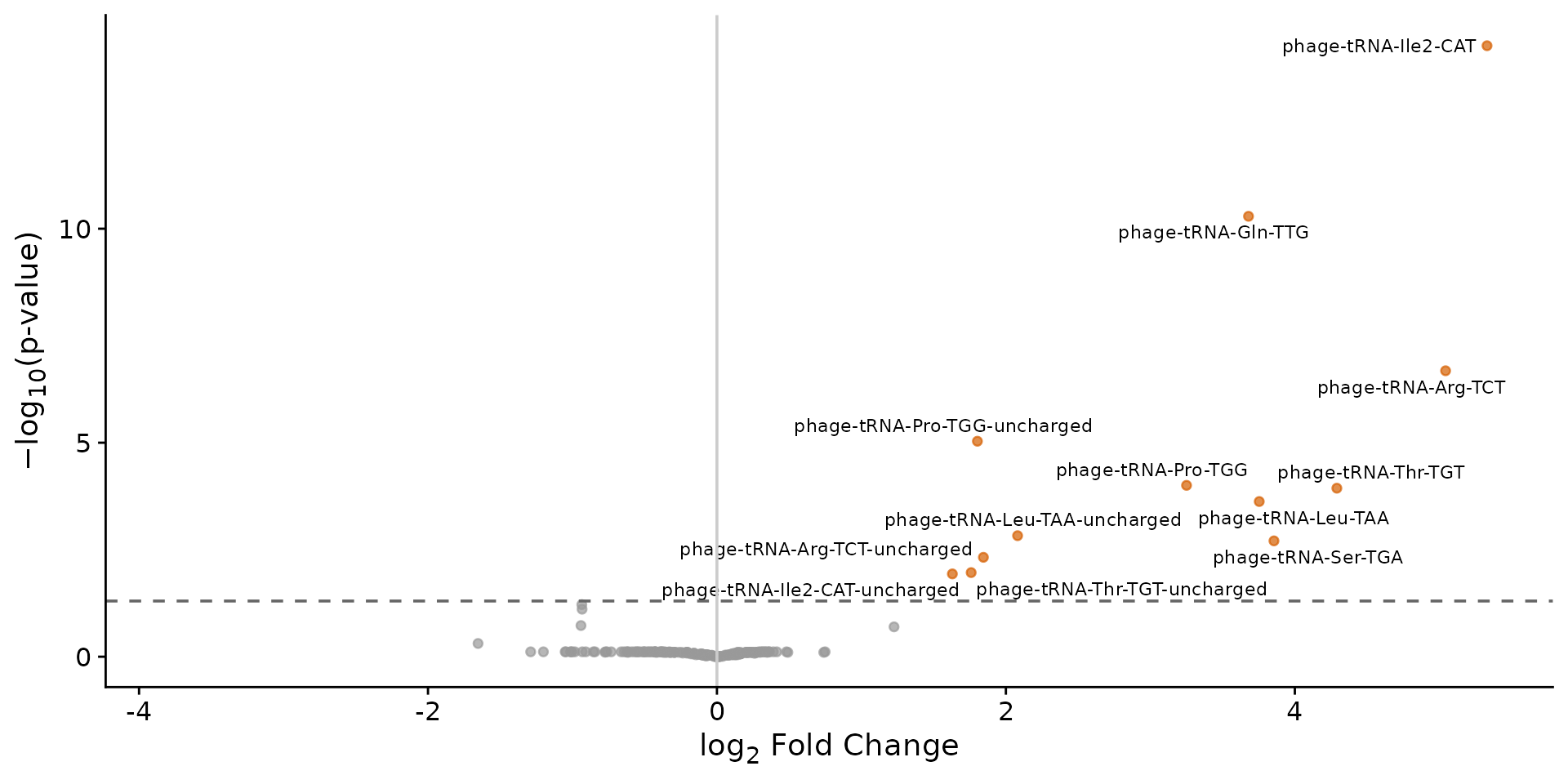
Volcano plot of differential tRNA abundance (inf vs ctl).
Differential charging analysis
A unique feature of nanopore tRNA-seq is the ability to measure charging levels. We can test whether the ratio of charged to uncharged reads changes upon infection.
charging <- metadata(se)$charging
charging$condition <- ifelse(grepl("ctl", charging$sample_id), "ctl", "inf")

ratio_diff <- compute_charging_diffs(
  charging,
  numerator = "inf",
  denominator = "ctl",
  min_count = 50,
  n_top = 20
)

plot_charging_diffs(ratio_diff)
Change in charging ratio (infected - control) per tRNA.
Abundance versus charging
We can visualize the relationship between abundance changes and charging ratio changes on a single scatter plot. This highlights tRNAs where expression and aminoacylation are coordinately or discordantly affected.
plot_abundance_charging(res, ratio_diff)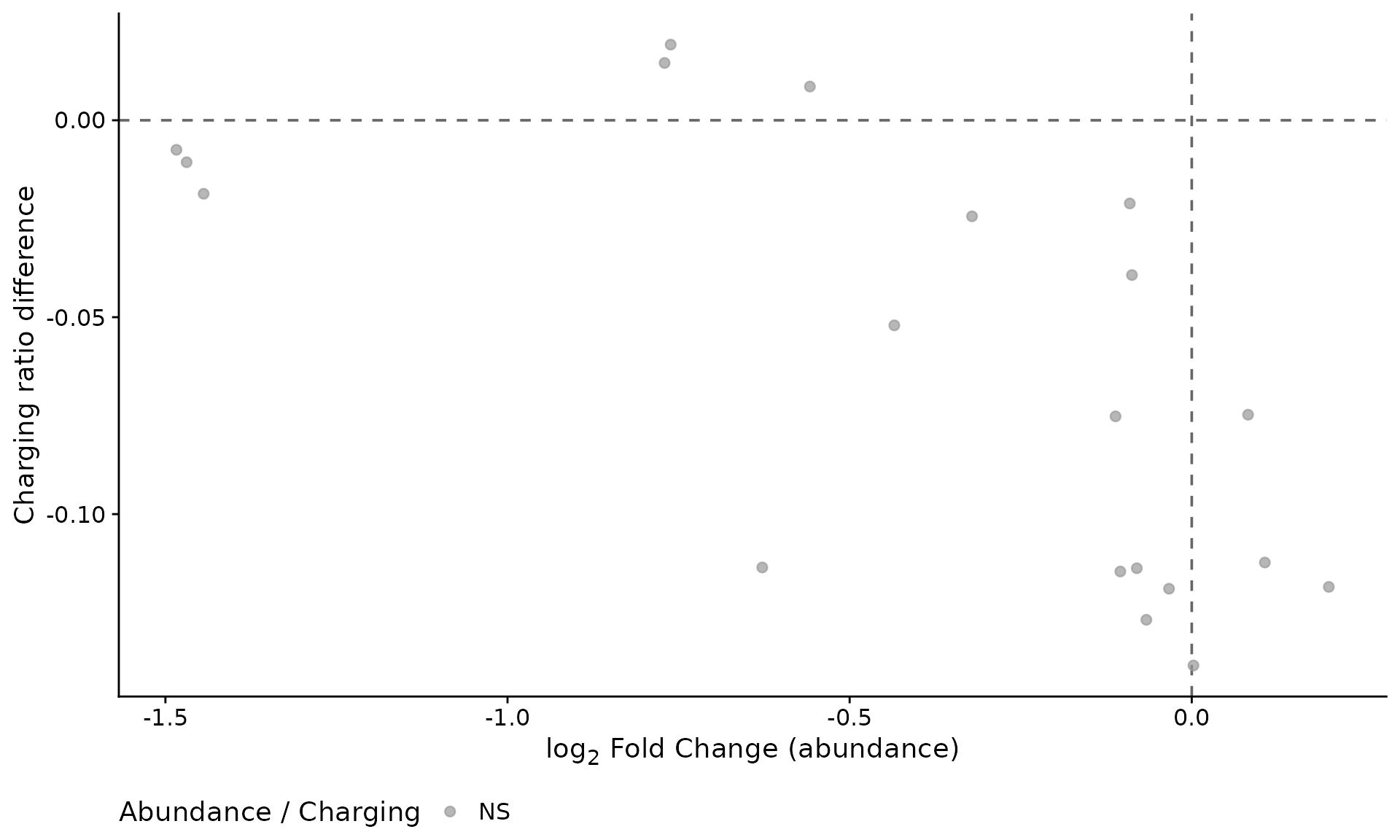
Abundance change versus charging ratio change per tRNA.
Base-calling error profiles
Base-calling error rates reflect RNA modifications that cause the nanopore basecaller to misidentify bases. Comparing error profiles between conditions can reveal modification changes.
# Load preprocessed bcerror data comparing wt vs TruB-del (tb) for 10 tRNAs
bcerror_rds <- readRDS(clover_example("ecoli/bcerror_summary.rds"))
bcerror_charged <- bcerror_rds$bcerror_charged
bcerror_summary <- bcerror_rds$bcerror_summary
# Plot error profiles for a few tRNAs
plot_trnas <- c(
  "host-tRNA-Asn-GTT-1-1",
  "host-tRNA-Glu-TTC-1-1",
  "host-tRNA-Phe-GAA-1-1"
)

plot_bcerror_profile(bcerror_summary, refs = plot_trnas)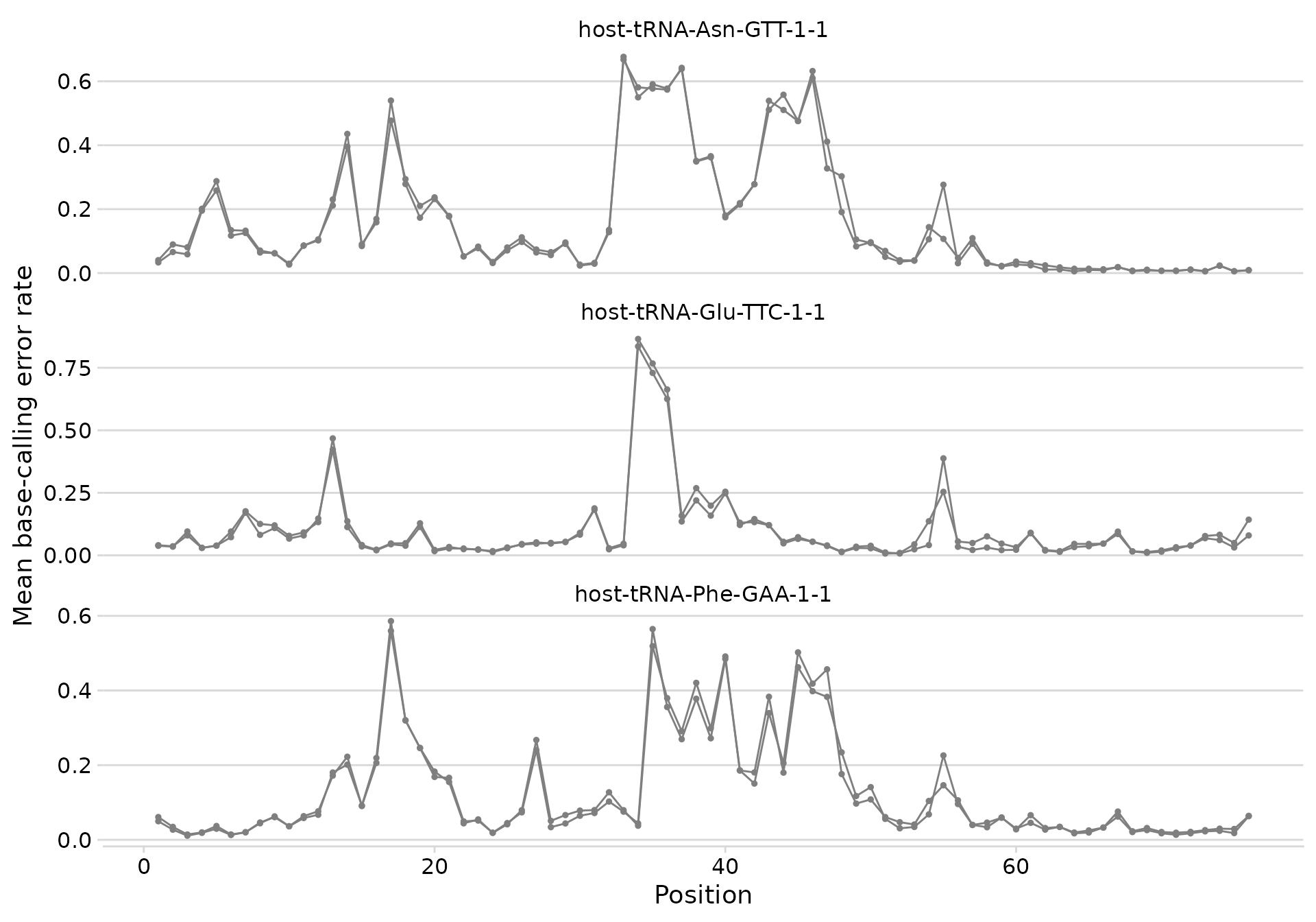
Base-calling error profiles for selected tRNAs.
Error rate difference heatmap
# Compute delta (wt - tb); positive = higher error in wt (modification present)
bcerror_delta <- compute_bcerror_delta(bcerror_summary, delta = wt - tb)

# Add Sprinzl coordinates and MODOMICS modification annotations
sprinzl <- read_sprinzl_coords(
  clover_example("sprinzl/ecoliK12_global_coords.tsv.gz")
)
trna_fasta <- clover_example("ecoli/trna_only.fa.gz")
mods <- modomics_mods(trna_fasta, organism = "Escherichia coli")

heatmap_data <- prep_mod_heatmap(
  bcerror_delta,
  sprinzl_coords = sprinzl,
  mods = mods
)

plot_mod_heatmap(
  heatmap_data,
  value_col = "delta",
  ref_col = "trna_label",
  cluster = FALSE,
  color_limits = c(-0.1, 0.1),
  highlight_col = "has_mod"
)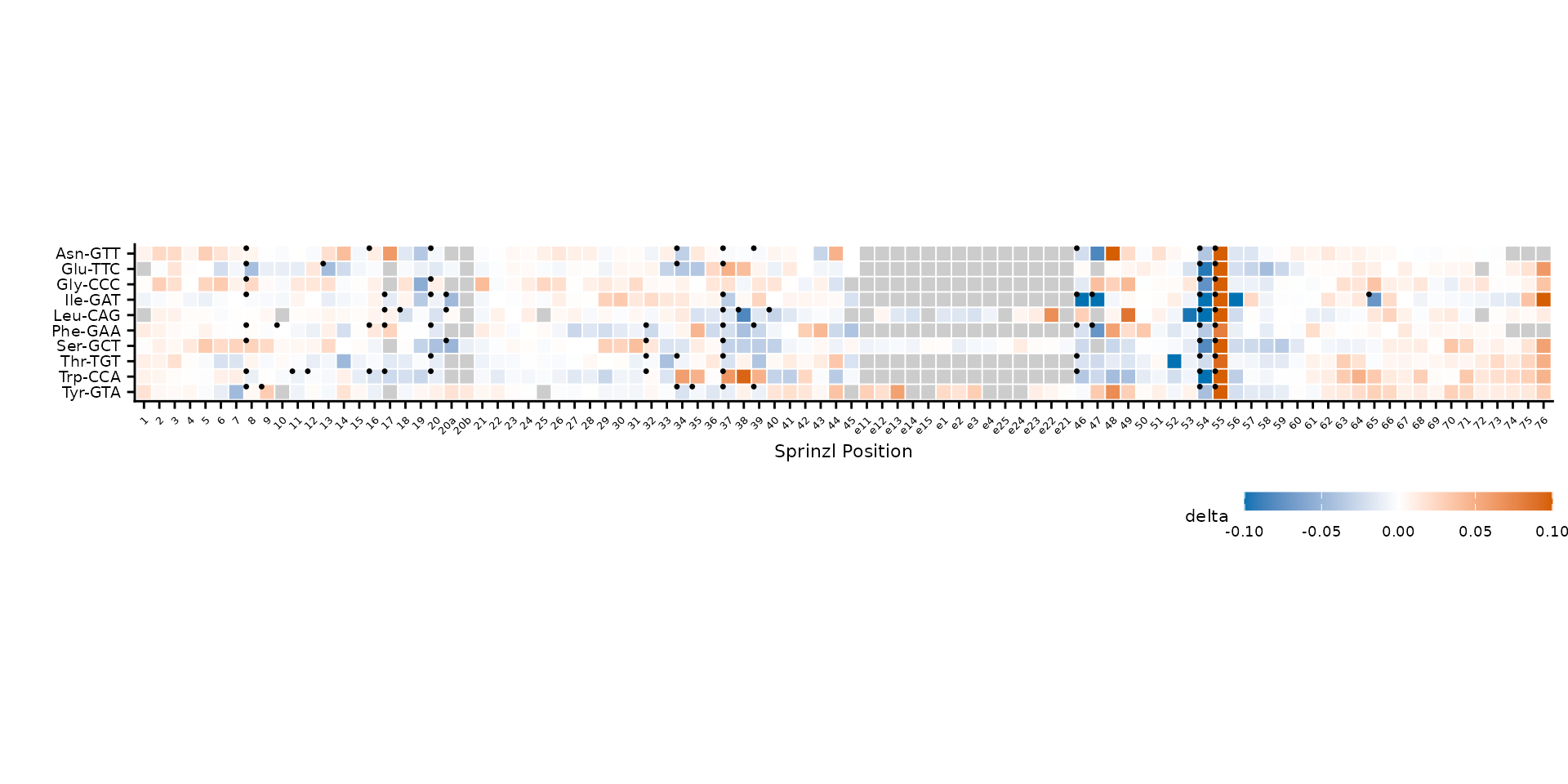
Difference in mean base-calling error (wt - TruB-del) across all tRNAs and positions.
Modification annotations from MODOMICS
The MODOMICS database
catalogs known RNA modifications. We already used
modomics_mods() above to annotate the heatmap with known
modification positions. This function maps MODOMICS entries onto your
reference sequences using pairwise alignment. Data for common organisms
is bundled with the package (see modomics_organisms()), so
no internet connection is needed.
mods
#> # A tibble: 701 × 4
#>    ref                     pos mod_full                 mod1
#>    <chr>                 <int> <chr>                    <chr>
#>  1 host-tRNA-Ala-TGC-1-1    17 dihydrouridine           D
#>  2 host-tRNA-Ala-TGC-1-1    34 uridine 5-oxyacetic acid cmo5U
#>  3 host-tRNA-Ala-TGC-1-1    46 7-methylguanosine        m7G
#>  4 host-tRNA-Ala-TGC-1-1    54 5-methyluridine          m5U
#>  5 host-tRNA-Ala-TGC-1-1    55 pseudouridine            Y
#>  6 host-tRNA-Ala-GGC-1-1    17 dihydrouridine           D
#>  7 host-tRNA-Ala-GGC-1-1    46 7-methylguanosine        m7G
#>  8 host-tRNA-Ala-GGC-1-1    54 5-methyluridine          m5U
#>  9 host-tRNA-Ala-GGC-1-1    55 pseudouridine            Y
#> 10 host-tRNA-Arg-ACG-1-1     8 4-thiouridine            s4U
#> # ℹ 691 more rows
We can overlay known modifications onto the base-calling error profiles. Positions with known modifications often correspond to elevated error rates, since the basecaller misidentifies modified nucleotides.
plot_bcerror_profile(bcerror_summary, refs = plot_trnas, mods = mods)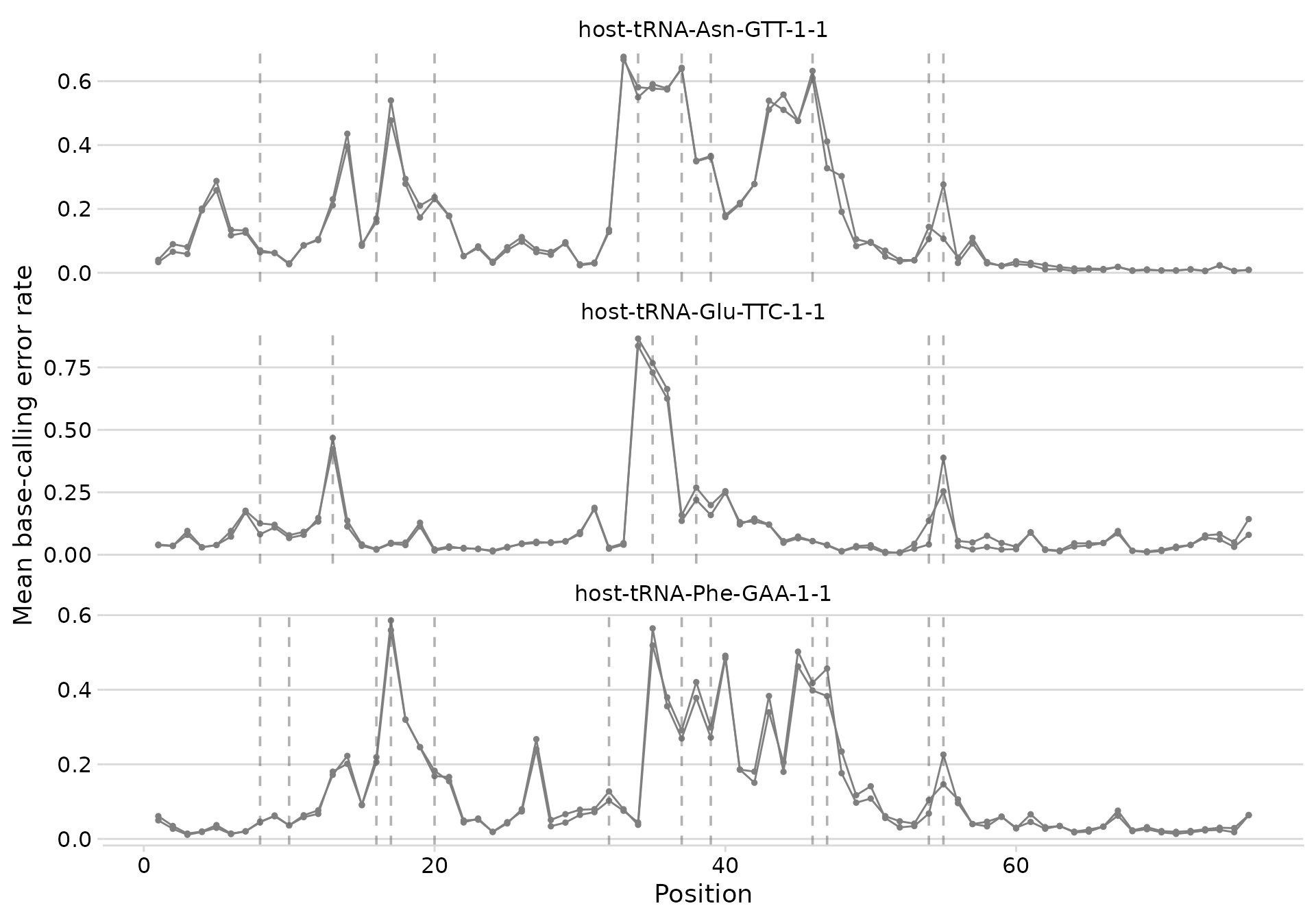
Base-calling error profiles with known modification positions marked.
tRNA secondary structure visualization
clover includes pre-computed tRNA cloverleaf SVGs for several model organisms. You can overlay modification annotations, circle outlines, and text color changes onto these structures.
# List available organisms and tRNAs
structure_organisms()
#> [1] "Escherichia coli"         "Homo sapiens"
#> [3] "Saccharomyces cerevisiae" "T4 phage"
head(structure_trnas("Escherichia coli"))
#> [1] "tRNA-Ala-GGC" "tRNA-Ala-TGC" "tRNA-Arg-ACG" "tRNA-Arg-CCG" "tRNA-Arg-CCT"
#> [6] "tRNA-Arg-TCT"
Base structure
The simplest call renders the bare cloverleaf with base-pair lines and nucleotide letters.
svg_path <- plot_tRNA_structure("tRNA-Glu-TTC", "Escherichia coli")Annotated structure with modifications, outlines, and text colors
We can highlight the anticodon with filled circles, mark the discriminator base with an outline, and change the text color of specific positions.
# Known modifications for this tRNA
mods_glu_struct <- mods |>
  filter(ref == "host-tRNA-Glu-TTC-1-1")

# Look up sequence positions for Sprinzl anticodon (34-36) and
# discriminator base (73)
glu_coords <- sprinzl |>
  filter(trna_id == "tRNA-Glu-UUC-1-1")

ac_pos <- glu_coords |>
  filter(sprinzl_label %in% c("34", "35", "36")) |>
  pull(pos)

disc_pos <- glu_coords |>
  filter(sprinzl_label == "73") |>
  pull(pos)

# Anticodon positions as filled circles
anticodon <- tibble::tibble(
  pos = ac_pos,
  mod1 = rep("anticodon", 3)
)

# Combine MODOMICS mods with anticodon highlight
all_mods <- bind_rows(mods_glu_struct, anticodon)

# Discriminator base as an outline
disc_outline <- tibble::tibble(pos = disc_pos, group = "discriminator")

# Change discriminator text to red
disc_text <- tibble::tibble(pos = disc_pos, color = "#E41A1C")

svg_path <- plot_tRNA_structure(
  "tRNA-Glu-TTC",
  "Escherichia coli",
  modifications = all_mods,
  mod_palette = c(default_mod_palette(), anticodon = "#4DAF4A"),
  outlines = disc_outline,
  outline_palette = c(discriminator = "#E41A1C"),
  text_colors = disc_text
)Long variable arm tRNAs
Leu and Ser tRNAs have a 4-stem cloverleaf with a variable arm stem, which is properly rendered from the tRNAscan-SE covariance model alignment.
svg_path <- plot_tRNA_structure("tRNA-Leu-CAA", "Escherichia coli")Modification co-occurrence on structure
We can visualize pairwise modification co-occurrence directly on the tRNA cloverleaf. Arcs connect position pairs with significant odds ratios: blue arcs indicate mutual exclusivity (negative log OR) and vermillion arcs indicate co-occurrence (positive log OR). Stroke width encodes the magnitude.
or_data <- metadata(se)$odds_ratios

# Filter OR data for one tRNA and one sample, clean, and filter for
# significance. filter_linkages() returns a tibble ready for plotting.
linkages_glu <- or_data |>
  filter(
    ref == "host-tRNA-Glu-TTC-1-1",
    sample_id == "wt-15-ctl-01"
  ) |>
  clean_odds_ratios() |>
  filter_linkages()

svg_path <- plot_tRNA_structure(
  "tRNA-Glu-TTC",
  "Escherichia coli",
  modifications = mods_glu_struct,
  linkages = linkages_glu
)Next steps
For isodecoder-level modification rewiring analysis — including odds ratio aggregation, ratio of odds ratios, dimensionality reduction, and network visualization — see the rewiring article.
Session info
sessionInfo()
#> R version 4.6.0 (2026-04-24)
#> Platform: x86_64-pc-linux-gnu
#> Running under: Ubuntu 24.04.4 LTS
#>
#> Matrix products: default
#> BLAS:   /usr/lib/x86_64-linux-gnu/openblas-pthread/libblas.so.3
#> LAPACK: /usr/lib/x86_64-linux-gnu/openblas-pthread/libopenblasp-r0.3.26.so;  LAPACK version 3.12.0
#>
#> locale:
#>  [1] LC_CTYPE=C.UTF-8       LC_NUMERIC=C           LC_TIME=C.UTF-8
#>  [4] LC_COLLATE=C.UTF-8     LC_MONETARY=C.UTF-8    LC_MESSAGES=C.UTF-8
#>  [7] LC_PAPER=C.UTF-8       LC_NAME=C              LC_ADDRESS=C
#> [10] LC_TELEPHONE=C         LC_MEASUREMENT=C.UTF-8 LC_IDENTIFICATION=C
#>
#> time zone: UTC
#> tzcode source: system (glibc)
#>
#> attached base packages:
#> [1] stats4    stats     graphics  grDevices utils     datasets  methods
#> [8] base
#>
#> other attached packages:
#>  [1] tidyr_1.3.2                 dplyr_1.2.1
#>  [3] SummarizedExperiment_1.42.0 Biobase_2.72.0
#>  [5] GenomicRanges_1.64.0        Seqinfo_1.2.0
#>  [7] IRanges_2.46.0              S4Vectors_0.50.1
#>  [9] BiocGenerics_0.58.1         generics_0.1.4
#> [11] MatrixGenerics_1.24.0       matrixStats_1.5.0
#> [13] clover_0.1.0.9000
#>
#> loaded via a namespace (and not attached):
#>  [1] tidyselect_1.2.1    farver_2.1.2        Biostrings_2.80.1
#>  [4] S7_0.2.2            fastmap_1.2.0       digest_0.6.39
#>  [7] lifecycle_1.0.5     pwalign_1.8.0       magrittr_2.0.5
#> [10] compiler_4.6.0      rlang_1.2.0         sass_0.4.10
#> [13] tools_4.6.0         utf8_1.2.6          yaml_2.3.12
#> [16] gt_1.3.0            knitr_1.51          S4Arrays_1.12.0
#> [19] labeling_0.4.3      htmlwidgets_1.6.4   bit_4.6.0
#> [22] DelayedArray_0.38.2 xml2_1.5.2          RColorBrewer_1.1-3
#> [25] abind_1.4-8         BiocParallel_1.46.0 withr_3.0.2
#> [28] purrr_1.2.2         desc_1.4.3          grid_4.6.0
#> [31] ggplot2_4.0.3       scales_1.4.0        cli_3.6.6
#> [34] rmarkdown_2.31      crayon_1.5.3        ragg_1.5.2
#> [37] tzdb_0.5.0          commonmark_2.0.0    cachem_1.1.0
#> [40] stringr_1.6.0       parallel_4.6.0      XVector_0.52.0
#> [43] vctrs_0.7.3         Matrix_1.7-5        jsonlite_2.0.0
#> [46] litedown_0.9        hms_1.1.4           bit64_4.8.2
#> [49] ggrepel_0.9.8       systemfonts_1.3.2   locfit_1.5-9.12
#> [52] jquerylib_0.1.4     glue_1.8.1          reactR_0.6.1
#> [55] pkgdown_2.2.0       codetools_0.2-20    ggtext_0.1.2
#> [58] cowplot_1.2.0       stringi_1.8.7       gtable_0.3.6
#> [61] tibble_3.3.1        pillar_1.11.1       htmltools_0.5.9
#> [64] reactable_0.4.5     R6_2.6.1            textshaping_1.0.5
#> [67] vroom_1.7.1         evaluate_1.0.5      lattice_0.22-9
#> [70] markdown_2.0        readr_2.2.0         gridtext_0.1.6
#> [73] bslib_0.11.0        Rcpp_1.1.1-1.1      SparseArray_1.12.2
#> [76] DESeq2_1.52.0       xfun_0.57           fs_2.1.0
#> [79] forcats_1.0.1       pkgconfig_2.0.3