Familiar tools, natively in R
The functions in valr have similar names to their
BEDtools counterparts, and so will be familiar to users
coming from the BEDtools suite. Similar to pybedtools,
valr has a terse syntax:
library(valr)
library(dplyr)

snps <- read_bed(valr_example("hg19.snps147.chr22.bed.gz"))
genes <- read_bed(valr_example("genes.hg19.chr22.bed.gz"))

# find snps in intergenic regions
intergenic <- bed_subtract(snps, genes)
# distance from intergenic snps to nearest gene
nearby <- bed_closest(intergenic, genes)

nearby |>
  select(starts_with("name"), .overlap, .dist) |>
  filter(abs(.dist) < 1000)
#> # A tibble: 555 × 4
#>    name.x      name.y            .overlap .dist
#>    <chr>       <chr>                <int> <int>
#>  1 rs2261631   P704P                    0  -268
#>  2 rs570770556 POTEH                    0  -913
#>  3 rs538163832 POTEH                    0  -953
#>  4 rs9606135   TPTEP1                   0  -422
#>  5 rs11912392  ANKRD62P1-PARP4P3        0   105
#>  6 rs555445266 ANKRD62P1-PARP4P3        0     1
#>  7 rs8136454   BC038197                 0   356
#>  8 rs576739562 XKR3                     0     1
#>  9 rs5992556   XKR3                     0  -456
#> 10 rs114101676 GAB4                     0   474
#> # ℹ 545 more rows
Input data
valr assigns common column names to facilitate
comparisons between tbls. All tbls will have chrom,
start, and end columns, and some tbls from
multi-column formats will have additional pre-determined column names.
See the read_bed() documentation for details.
bed_file <- valr_example("3fields.bed.gz")
read_bed(bed_file) # accepts filepaths or URLs
#> # A tibble: 10 × 3
#>    chrom  start    end
#>    <chr>  <dbl>  <dbl>
#>  1 chr1   11873  14409
#>  2 chr1   14361  19759
#>  3 chr1   14406  29370
#>  4 chr1   34610  36081
#>  5 chr1   69090  70008
#>  6 chr1  134772 140566
#>  7 chr1  321083 321115
#>  8 chr1  321145 321207
#>  9 chr1  322036 326938
#> 10 chr1  327545 328439
valr can also operate on BED-like data.frames already
constructed in R, provided that columns named chrom,
start and end are present. New tbls can also
be constructed as either tibbles or base R
data.frames.
bed <- tribble(
  ~chrom , ~start  , ~end    ,
  "chr1" , 1657492 , 2657492 ,
  "chr2" , 2501324 , 3094650
)

bed
#> # A tibble: 2 × 3
#>   chrom   start     end
#>   <chr>   <dbl>   <dbl>
#> 1 chr1  1657492 2657492
#> 2 chr2  2501324 3094650
bigWig and bigBed files
Signal (bigWig) and feature (bigBed) files are read with
read_bigwig() and read_bigbed(), which accept
local paths or http(s):// URLs.
bw <- valr_example("hg19.dnase1.bw")
read_bigwig(bw)
#> # A tibble: 2,587 × 4
#>    chrom    start      end value
#>    <chr>    <int>    <int> <dbl>
#>  1 chr22 16050284 16050464     1
#>  2 chr22 16051024 16051204     1
#>  3 chr22 16051224 16051764     1
#>  4 chr22 16052724 16052904     1
#>  5 chr22 16053224 16053404     1
#>  6 chr22 16054584 16054644     1
#>  7 chr22 16054644 16054764     2
#>  8 chr22 16054764 16054824     1
#>  9 chr22 16056404 16056424     1
#> 10 chr22 16056424 16056584     2
#> # ℹ 2,577 more rows
The multiple-set operations (bed_intersect(),
bed_map(), bed_coverage(),
bed_subtract(), and bed_window()) also accept
a bigWig or bigBed path or URL directly in place of a y
tbl. Only the regions spanned by x are read from the file,
so large (and remote) files are queried without loading them in
full.
peaks <- tribble(
  ~chrom , ~start    , ~end      ,
  "chr22", 16100000  , 16150000  ,
  "chr22", 16500000  , 16550000
)

# sum DNase I signal over each peak, reading only those regions from the file
bed_map(peaks, bw, .signal = sum(value))
#> # A tibble: 2 × 4
#>   chrom    start      end .signal
#>   <chr>    <dbl>    <dbl>   <dbl>
#> 1 chr22 16100000 16150000     101
#> 2 chr22 16500000 16550000      17
Interval coordinates
valr adheres to the BED format which
specifies that the start position for an interval is zero based and the
end position is one-based. The first position in a chromosome is 0. The
end position for a chromosome is one position passed the last base, and
is not included in the interval. For example:
# a chromosome 100 basepairs in length
chrom <- tribble(
  ~chrom , ~start , ~end ,
  "chr1" ,      0 ,  100
)

chrom
#> # A tibble: 1 × 3
#>   chrom start   end
#>   <chr> <dbl> <dbl>
#> 1 chr1      0   100

# single base-pair intervals
bases <- tribble(
  ~chrom , ~start , ~end ,
  "chr1" ,      0 ,    1 , # first base of chromosome
  "chr1" ,      1 ,    2 , # second base of chromosome
  "chr1" ,     99 ,  100 # last base of chromosome
)

bases
#> # A tibble: 3 × 3
#>   chrom start   end
#>   <chr> <dbl> <dbl>
#> 1 chr1      0     1
#> 2 chr1      1     2
#> 3 chr1     99   100
Remote databases
Remote databases can be accessed with db_ucsc() (to
access the UCSC Browser) and db_ensembl() (to access
Ensembl databases).
Visual documentation
The bed_glyph() tool illustrates the results of
operations in valr, similar to those found in the
BEDtools documentation. This glyph shows the result of
intersecting x and y intervals with
bed_intersect():
x <- tribble(
  ~chrom , ~start , ~end ,
  "chr1" ,     25 ,   50 ,
  "chr1" ,    100 ,  125
)

y <- tribble(
  ~chrom , ~start , ~end ,
  "chr1" ,     30 ,   75
)

bed_glyph(bed_intersect(x, y))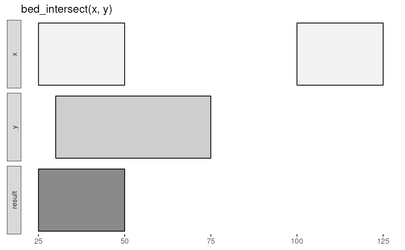
And this glyph illustrates bed_merge():
x <- tribble(
  ~chrom , ~start , ~end ,
  "chr1" ,      1 ,   50 ,
  "chr1" ,     10 ,   75 ,
  "chr1" ,    100 ,  120
)

bed_glyph(bed_merge(x))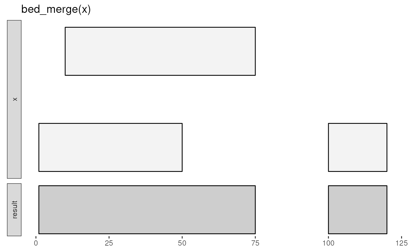
Grouping data
The group_by function in dplyr can be used to perform
functions on subsets of single and multiple data_frames.
Functions in valr leverage grouping to enable a variety of
comparisons. For example, intervals can be grouped by
strand to perform comparisons among intervals on the same
strand.
x <- tribble(
  ~chrom , ~start , ~end , ~strand ,
  "chr1" ,      1 ,  100 , "+"     ,
  "chr1" ,     50 ,  150 , "+"     ,
  "chr2" ,    100 ,  200 , "-"
)

y <- tribble(
  ~chrom , ~start , ~end , ~strand ,
  "chr1" ,     50 ,  125 , "+"     ,
  "chr1" ,     50 ,  150 , "-"     ,
  "chr2" ,     50 ,  150 , "+"
)

# intersect tbls by strand
x <- group_by(x, strand)
y <- group_by(y, strand)

bed_intersect(x, y)
#> # A tibble: 2 × 8
#>   chrom start.x end.x strand.x start.y end.y strand.y .overlap
#>   <chr>   <dbl> <dbl> <chr>      <dbl> <dbl> <chr>       <int>
#> 1 chr1        1   100 +             50   125 +              50
#> 2 chr1       50   150 +             50   125 +              75
Comparisons between intervals on opposite strands are done using the
flip_strands() function:
x <- group_by(x, strand)

y <- flip_strands(y)
y <- group_by(y, strand)

bed_intersect(x, y)
#> # A tibble: 3 × 8
#>   chrom start.x end.x strand.x start.y end.y strand.y .overlap
#>   <chr>   <dbl> <dbl> <chr>      <dbl> <dbl> <chr>       <int>
#> 1 chr1        1   100 +             50   150 +              50
#> 2 chr1       50   150 +             50   150 +             100
#> 3 chr2      100   200 -             50   150 -              50
Both single set (e.g. bed_merge()) and multi set
operations will respect groupings in the input intervals.
Column specification
Columns in BEDtools are referred to by position:
# calculate the mean of column 6 for intervals in `b` that overlap with `a`
bedtools map -a a.bed -b b.bed -c 6 -o mean
In valr, columns are referred to by name and can be used
in multiple name/value expressions for summaries.
Getting started
Meta-analysis
This demonstration illustrates how to use valr tools to
perform a “meta-analysis” of signals relative to genomic features. Here
we to analyze the distribution of histone marks surrounding
transcription start sites.
First we load libraries and relevant data.
# `valr_example()` identifies the path of example files
bedfile <- valr_example("genes.hg19.chr22.bed.gz")
genomefile <- valr_example("hg19.chrom.sizes.gz")
bgfile <- valr_example("hela.h3k4.chip.bg.gz")

genes <- read_bed(bedfile)
genome <- read_genome(genomefile)
y <- read_bedgraph(bgfile)
Then we generate 1 bp intervals to represent transcription start
sites (TSSs). We focus on + strand genes, but
- genes are easily accommodated by filtering them and using
bed_makewindows() with reversed window
numbers.
# generate 1 bp TSS intervals, `+` strand only
tss <- genes |>
  filter(strand == "+") |>
  mutate(end = start + 1)

# 1000 bp up and downstream
region_size <- 1000
# 50 bp windows
win_size <- 50

# add slop to the TSS, break into windows and add a group
x <- tss |>
  bed_slop(genome, both = region_size) |>
  bed_makewindows(win_size)

x
#> # A tibble: 13,530 × 7
#>    chrom    start      end name      score strand .win_id
#>    <chr>    <dbl>    <dbl> <chr>     <chr> <chr>    <int>
#>  1 chr22 16161065 16161115 LINC00516 3     +            1
#>  2 chr22 16161115 16161165 LINC00516 3     +            2
#>  3 chr22 16161165 16161215 LINC00516 3     +            3
#>  4 chr22 16161215 16161265 LINC00516 3     +            4
#>  5 chr22 16161265 16161315 LINC00516 3     +            5
#>  6 chr22 16161315 16161365 LINC00516 3     +            6
#>  7 chr22 16161365 16161415 LINC00516 3     +            7
#>  8 chr22 16161415 16161465 LINC00516 3     +            8
#>  9 chr22 16161465 16161515 LINC00516 3     +            9
#> 10 chr22 16161515 16161565 LINC00516 3     +           10
#> # ℹ 13,520 more rows
Now we use the .win_id group with bed_map()
to calculate a sum by mapping y signals onto the intervals
in x. These data are regrouped by .win_id and
a summary with mean and sd values is
calculated.
# map signals to TSS regions and calculate summary statistics.
res <- bed_map(x, y, win_sum = sum(value, na.rm = TRUE)) |>
  group_by(.win_id) |>
  summarize(
    win_mean = mean(win_sum, na.rm = TRUE),
    win_sd = sd(win_sum, na.rm = TRUE)
  )

res
#> # A tibble: 41 × 3
#>    .win_id win_mean win_sd
#>      <int>    <dbl>  <dbl>
#>  1       1     101.   85.8
#>  2       2     111.   81.1
#>  3       3     123.   99.1
#>  4       4     116.   96.3
#>  5       5     116.  102.
#>  6       6     125.   95.1
#>  7       7     123.   94.4
#>  8       8     128.   91.5
#>  9       9     130.   95.7
#> 10      10     130.   88.8
#> # ℹ 31 more rows
Finally, these summary statistics are used to construct a plot that illustrates histone density surrounding TSSs.
x_labels <- seq(
  -region_size,
  region_size,
  by = win_size * 5
)

x_breaks <- seq(1, 41, by = 5)

sd_limits <- aes(
  ymax = win_mean + win_sd,
  ymin = win_mean - win_sd
)

ggplot(
  res,
  aes(
    x = .win_id,
    y = win_mean
  )
) +
  geom_point() +
  geom_pointrange(sd_limits) +
  scale_x_continuous(
    labels = x_labels,
    breaks = x_breaks
  ) +
  labs(
    x = "Position (bp from TSS)",
    y = "Signal",
    title = "Human H3K4me3 signal near transcription start sites"
  ) +
  theme_classic()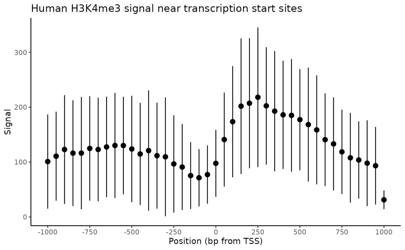
Related work
The Python library pybedtools wraps BEDtools.
The R packages GenomicRanges, bedr, IRanges and GenometriCorr provide similar capability with a different philosophy.