Single cell dataset alignment and batch correction
- Inter-sample variation can complicate the analysis of single cell data.
- This variation can include experimental or sequencing batch effects, technology-specific biases, experimental conditions, etc.
- Robust methods are available to align datasets from different platforms, experimental conditions, individuals and even species.
Packages covered:
- Harmony (https://github.com/immunogenomics/harmony)
- Seurat (https://satijalab.org/seurat/v3.0/integration.html)
- scAlign (https://github.com/quon-titative-biology/scAlign)
An example: Four pancreatic islet datasets
The code below downloads a Seurat object that contains human pancreatic islet cell data from four single cell sequencing technologies, CelSeq (GSE81076), CelSeq2 (GSE85241), Fluidigm C1 (GSE86469), and SMART-Seq2 (E-MTAB-5061). Basic QC and normalization has been performed, as described earlier in this workshop. The UMAP projections below illustrates the challenge: despite containing the same cell populations, the cells are separated not only by cell type (1st plot), but also by technology (2nd plot).
so <- readRDS(gzcon(url("https://scrnaseq-workshop.s3-us-west-2.amazonaws.com/pancreas.Rds")))

pre_cell_plot <- DimPlot(so,
                         reduction = "umap",
                         group.by = "celltype")
pre_tech_plot <- DimPlot(so,
                         reduction = "umap",
                         group.by = "tech")

plot_grid(pre_cell_plot,
          pre_tech_plot,
          nrow = 2)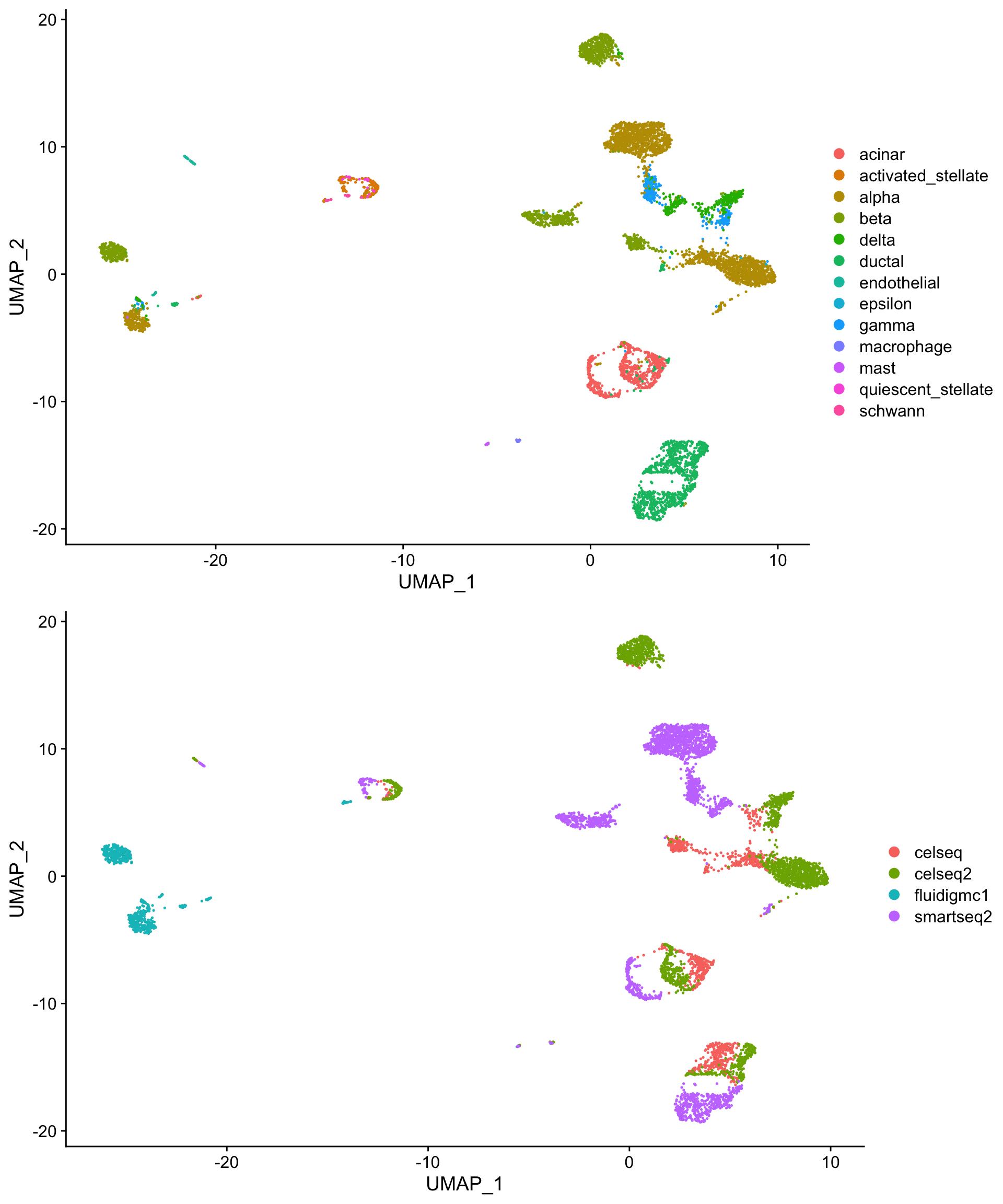
Quick and Flexible: Harmony

Harmony works by weakly clustering cells and then calculating - and iteratively refining - a dataset correction factor for each cluster. Note that Harmony only computes a new corrected dimensionality reduction - it does not calculate corrected expression values (the raw.data, data and scale.data slots are unmodified). This works well for most datasets, but can be be insufficient for downstream differential expression analyses in extremely divergent samples.
Running harmony on a Seurat object
Harmony provides a wrapper function (RunHarmony()) that can take Seurat (v2 or v3) or SingleCellExperiment objects directly. Here, we run harmony with the default parameters and generate a plot to confirm convergence. RunHarmony() returns an object with a new dimensionality reduction - named harmony - that can be used for downstream projections and clustering.
so <- RunHarmony(so,
                 group.by.vars = "tech",
                 plot_convergence = T)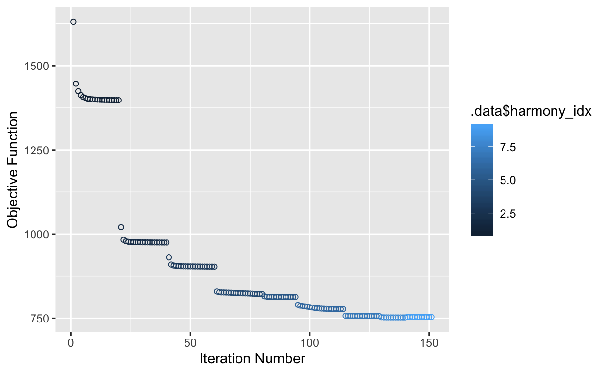
# a new reduction now appears, in the form of 'harmony'
so@reductions$harmony
#> A dimensional reduction object with key harmony_
#>  Number of dimensions: 50
#>  Projected dimensional reduction calculated:  TRUE
#>  Jackstraw run: FALSE
#>  Computed using assay: RNA
We can plot this new reduction directly, or use it to generate new UMAPs.
Plotting the first two harmony dimensions directly already reveals the value of this approach - the cells are now spatially clustered by cell type, rather than by technology:
harmony_cell_plot <- DimPlot(so,
                             reduction = "harmony",
                             group.by = "celltype")
harmony_tech_plot <- DimPlot(so,
                             reduction = "harmony",
                             group.by = "tech")

plot_grid(harmony_cell_plot,
          harmony_tech_plot,
          nrow = 2)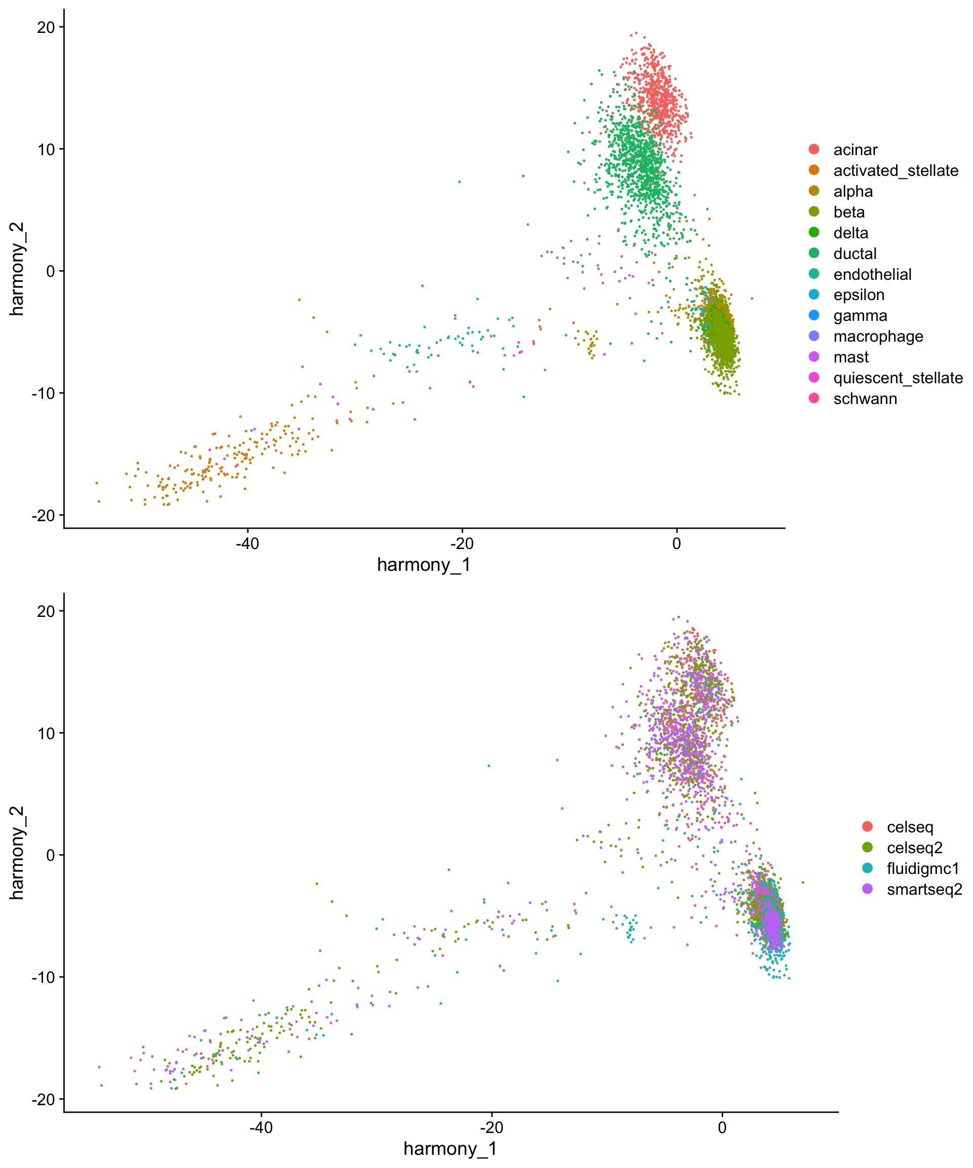
We can also generate UMAP projections from the harmony reductions.
# the first 20 harmony dimensions are a sane default
so <- RunUMAP(so,
              reduction = "harmony",
              dims = 1:20,
              reduction.name = "harmony_umap")

h_umap_cell_plot <- DimPlot(so,
                            reduction = "harmony_umap",
                            group.by = "celltype",
                            label = T,
                            repel = T)
h_umap_tech_plot <- DimPlot(so,
                            reduction = "harmony_umap",
                            group.by = "tech")

plot_grid(h_umap_cell_plot,
          h_umap_tech_plot,
          nrow = 2)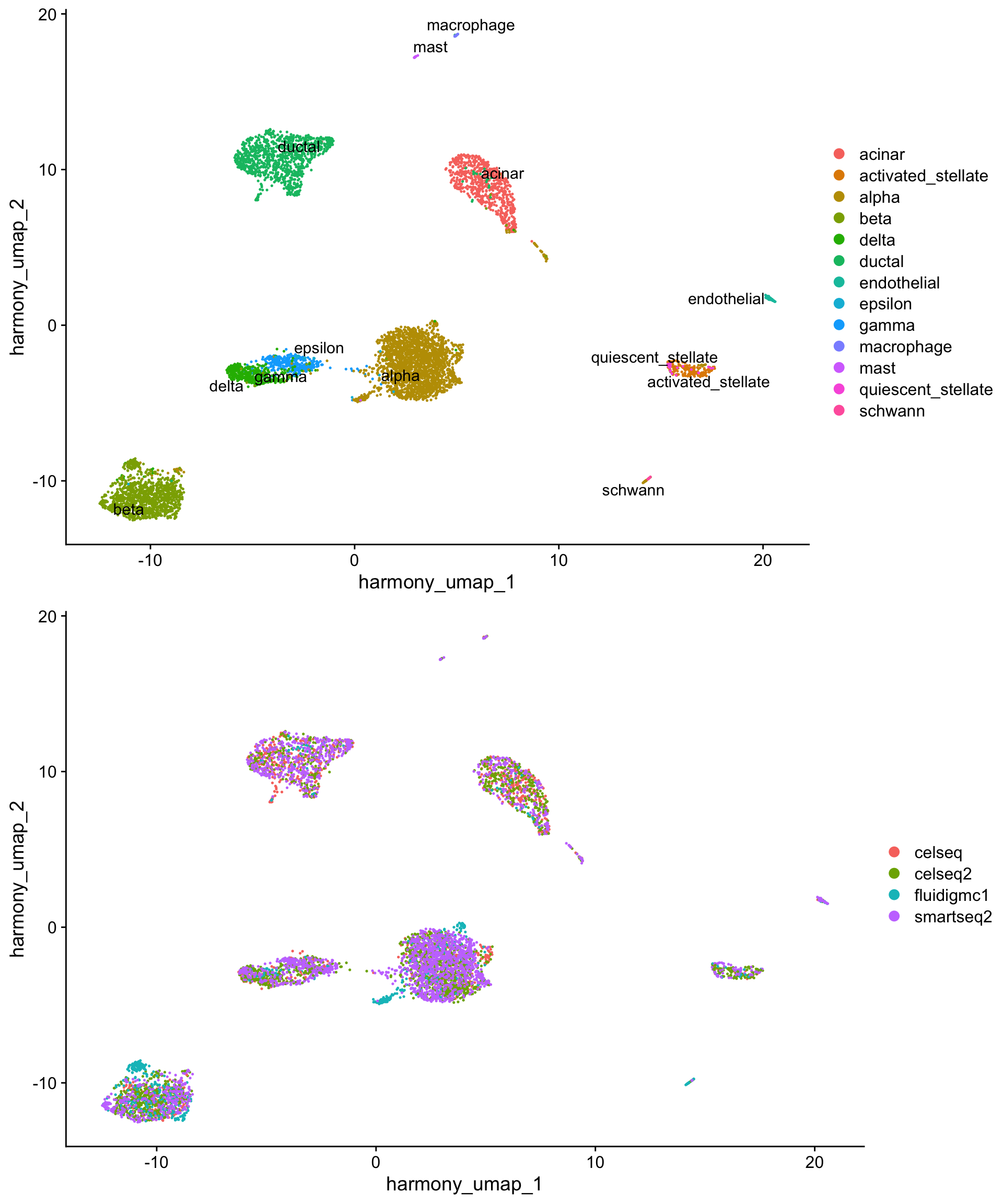
In this example, we already have labeled clusters in all four samples to simplify alignment quality assessment. In a production analysis, you will likely want to cluster the aligned cells using the harmony alignment. This is accomplished by providing reduction = "harmony" to FindNeighbors().
so <- FindNeighbors(so,
                    reduction = "harmony",
                    dims = 1:20)

so <- FindClusters(so,
                   resolution = 0.5)
Harmony is also highly tunable. Additional co-variates can be included and the strength of alignment can be tuned for each co-variate using the theta argument. Higher theta values result in more aggressive correction factors and, consequently, more aggressive dataset integration.
so <- RunHarmony(so,
                 group.by.vars = c("tech", ...), # can be any metadata column
                 theta = c(3,4)) # default theta = 2; higher value = more agressive integration
Built-in, but more complex to run: Seurat (v3) Integration

Seurat’s built-in integration works by identifying ‘anchors’ between pairs of datasets. These anchors represent pairwise correspondences between individual cells (one in each dataset) that originate from the same biological state. These ‘anchors’ are then used to harmonize the datasets. Unlike Harmony, Seruat’s integration approach does calculate corrected expression values.
Running Seurat v3 Integration
Adapted from the Seurat ‘standard workflow’ integration vignette.
To construct a reference, we first identify ‘anchors’ between the individual datasets. Unlike Harmony, Seurat requires that the datasets be in separate Seurat objects, so we split the object into a list of Seurat objects by technology used.
so.list <- SplitObject(so, split.by = "tech")Next, we perform standard preprocessing (log-normalization) on each individual object, and identify variable features in each.
seurat.preprocess <- function(so){
  so_tmp <- NormalizeData(so,
                          verbose = FALSE)
  so_tmp <- FindVariableFeatures(so_tmp,
                                 selection.method = "vst",
        nfeatures = 2000,
        verbose = FALSE)
  so_tmp
}

so.list <- map(so.list, ~seurat.preprocess(.x))
We will identify anchors using the FindIntegrationAnchors() function, which takes a list of Seurat objects as input. Here, we integrate our four objects into a reference.
We use all default parameters here, but Seurat integration is very flexible. In a production analysis, it can be useful to vary the ‘dimensionality’ of the dataset (default = ) over a broad range (e.g. 10-50) to determine the optimal anchor parameters. Also, if any dataset contains fewer than 200 cells, k.filter (the number of neighbors to use when filtering anchors) will need to be lowered. As an aside, this integration strategy does not work particularly well with small datasets (too few anchors).
so.anchors <- FindIntegrationAnchors(object.list = so.list,
                                     dims = 1:30, )
After identifying anchors, we run the IntegrateData function, which returns a single integrated Seurat object that contains a new Assay (“integrated”), which holds an integrated (‘batch-corrected’) expression matrix for all cells.
so.integrated <- IntegrateData(anchorset = so.anchors,
                               dims = 1:30)
We can then use this integrated matrix for downstream analysis and visualization exactly as described earlier in this workshop.
# switch to integrated assay. The variable features of this assay are automatically
# set during IntegrateData
DefaultAssay(so.integrated) <- "integrated"

# Run the standard workflow for visualization and clustering
so.integrated <- ScaleData(so.integrated,
                           verbose = FALSE)
so.integrated <- RunPCA(so.integrated,
                        npcs = 30,
                        verbose = FALSE)
so.integrated <- RunUMAP(so.integrated,
                         reduction = "pca",
                         dims = 1:30)
s_umap_cell_plot <- DimPlot(so.integrated,
                            reduction = "umap",
                            group.by = "celltype",
                            label = T,
                            repel = T)
s_umap_tech_plot <- DimPlot(so.integrated,
                            reduction = "umap",
                            group.by = "tech")

plot_grid(s_umap_cell_plot,
          s_umap_tech_plot,
          nrow = 2)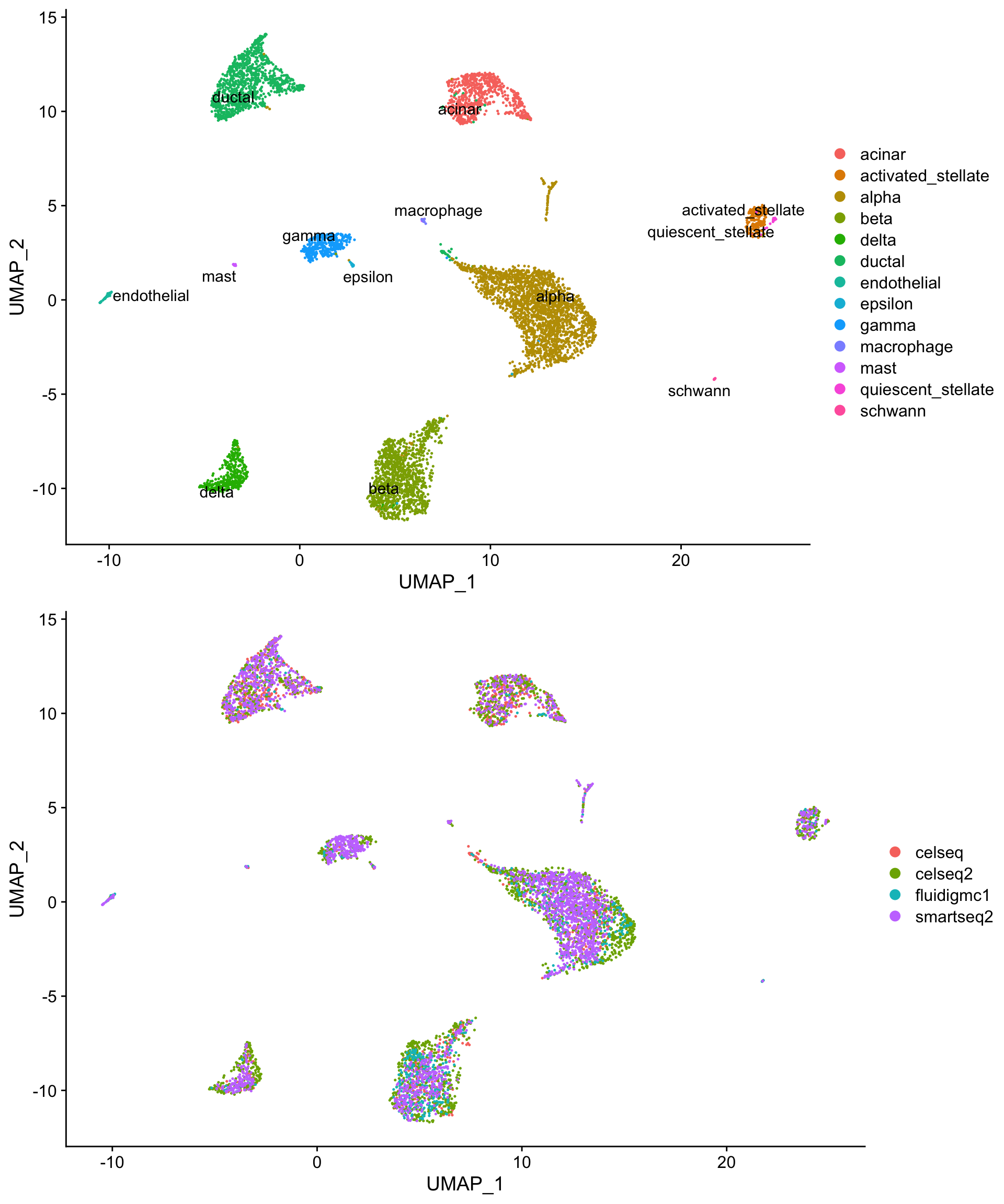
Deep learning: scAlign
scAlign uses a shared deep neural network to project cells into a shared expression or reduction space. This approach combines features of Harmony (new projections without modifying expression data) and Seurat (the ability to generate corrected expression matrices) with additional functionality that may be useful for some samples. Notably, scAlign can identify rare cell types/states across samples without the need to cluster the cells first. scAlign can also make use of existing labelled clusters in the source datasets (“supervised” mode) to improve integration.
Running scAlign on a Seurat object
Adapted from the scAlign vignettes.
Starting from the so.list we generated for the Seurat integration, we can jump right into the scAlign workflow.
scalign.preprocess <- function(so){
    so_tmp <- NormalizeData(so)
    so_tmp <- ScaleData(so_tmp,
                        features = rownames(so_tmp))
    so_tmp <- FindVariableFeatures(so_tmp,
                                   selection.method = "vst",
                                   nfeatures = 3000)
  so_tmp
}

so.list <- map(so.list,
               ~scalign.preprocess(.x))
Next, we can extract a common set of genes across all datasets.
genes.use <- unique(unlist(map(so.list,
                               ~.x@assays$RNA@var.features)))
The general design of scAlign makes it agnostic to the input RNA-seq data representation. Thus, the input data can either be gene-level counts, transformations of those gene level counts or a preliminary step of dimensionality reduction such as canonical correlates, principal component scores, or Harmony projections. Here we convert the previously defined Seurat objects to SingleCellExperiment objects in order to create the combined scAlign object.
so.sce.list = lapply(so.list,
                           function(seurat.obj){
                             SingleCellExperiment(assays = list(logcounts = seurat.obj@assays$RNA@data[genes.use,],
                                                                scale.data = seurat.obj@assays$RNA@scale.data[genes.use,]),
                                                  colData = seurat.obj@meta.data)
                            })
Next, we build the scAlign combined SCE object and append the results of the Harmony integration. The scAlign vignette uses the Seurat v2 RunMultiCCA reduction here, but the principle is the same (an intermediate dimensionality reduction in a shared projection space). Any shared metric can be used - log-space gene expression, PCA, CCA, etc.
scAlignPancreas = scAlignCreateObject(sce.objects = so.sce.list,
                                      project.name = "scAlign_Pancreatic_Islet",
                                      labels = map(so.sce.list,
                                                   ~.x@colData$celltype))

# the bracketed-subsetting ensures that the cell order is correct in the SCE object
reducedDim(scAlignPancreas, "Harmony") = so@reductions$harmony@cell.embeddings[rownames(scAlignPancreas@colData),]
Finally, we align the pancreas islets sequenced across different protocols using the results of RunHarmony as input to scAlign. This should not be run interactively during the workshop, as it is time consuming.
scAlignPancreas = scAlignMulti(scAlignPancreas,
                        options=scAlignOptions(steps=15000,
                                               log.every=5000,
                                               architecture="large",   ## 3 layer neural network
                                               num.dim=64),            ## Number of latent dimensions
                        encoder.data="Harmony",
                        supervised='none',
                        run.encoder=TRUE,
                        run.decoder=FALSE,
                        log.results=TRUE,
                        log.dir=file.path('./tmp'),
                        device = "GPU")

# convert the scAlign ovject to Seurat and run UMAP on the aligned reduction.
so.sca <- RunUMAP(as.Seurat(scAlignPancreas,
                            counts = NULL),
                  reduction = "ALIGNED-Harmony",
                  dims = 1:20)

# save the aligned Seurat object for plotting
saveRDS(so.sca, "so_sca.Rds")
As with Harmony and Seurat, scAlign produces a single, well-aligned projection. This is not a particularly compelling example of scAlign’s output - it’s built on Harmony’s output, after all - but is included primarily to demonstrate the scAlign workflow.
so.sca <- readRDS("so_sca.Rds")

sca_umap_cell_plot <- DimPlot(so.sca,
                              reduction = "umap",
                              group.by = "celltype",
                              label = T,
                              repel = T)
sca_umap_tech_plot <- DimPlot(so.sca,
                              reduction = "umap",
                              group.by = "tech")

plot_grid(sca_umap_cell_plot,
          sca_umap_tech_plot,
          nrow = 2)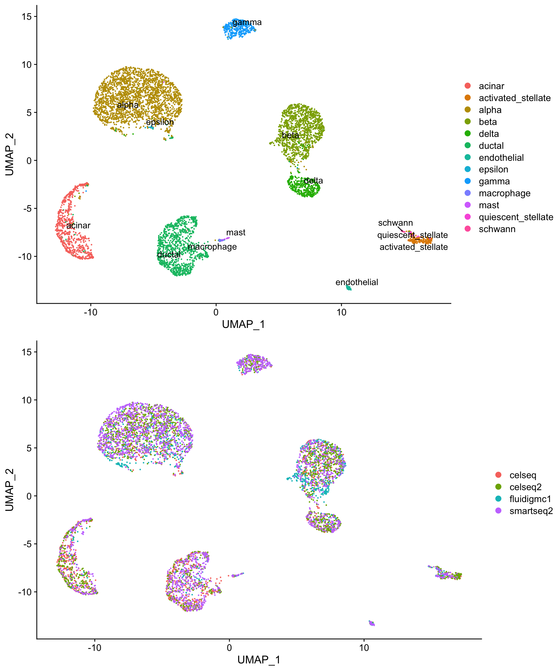
Comparing all three integration methods
All three integration/alignment methods do a similar job of aligning shared cell types across the four sequencing techniques.
CombinePlots(list(pre_cell_plot + ggtitle("Unaligned"),
                  h_umap_cell_plot + ggtitle("Harmony"),
                  s_umap_cell_plot + ggtitle("Seurat"),
                  sca_umap_cell_plot + ggtitle("scAlign")),
             legend = "none",
             ncol = 2)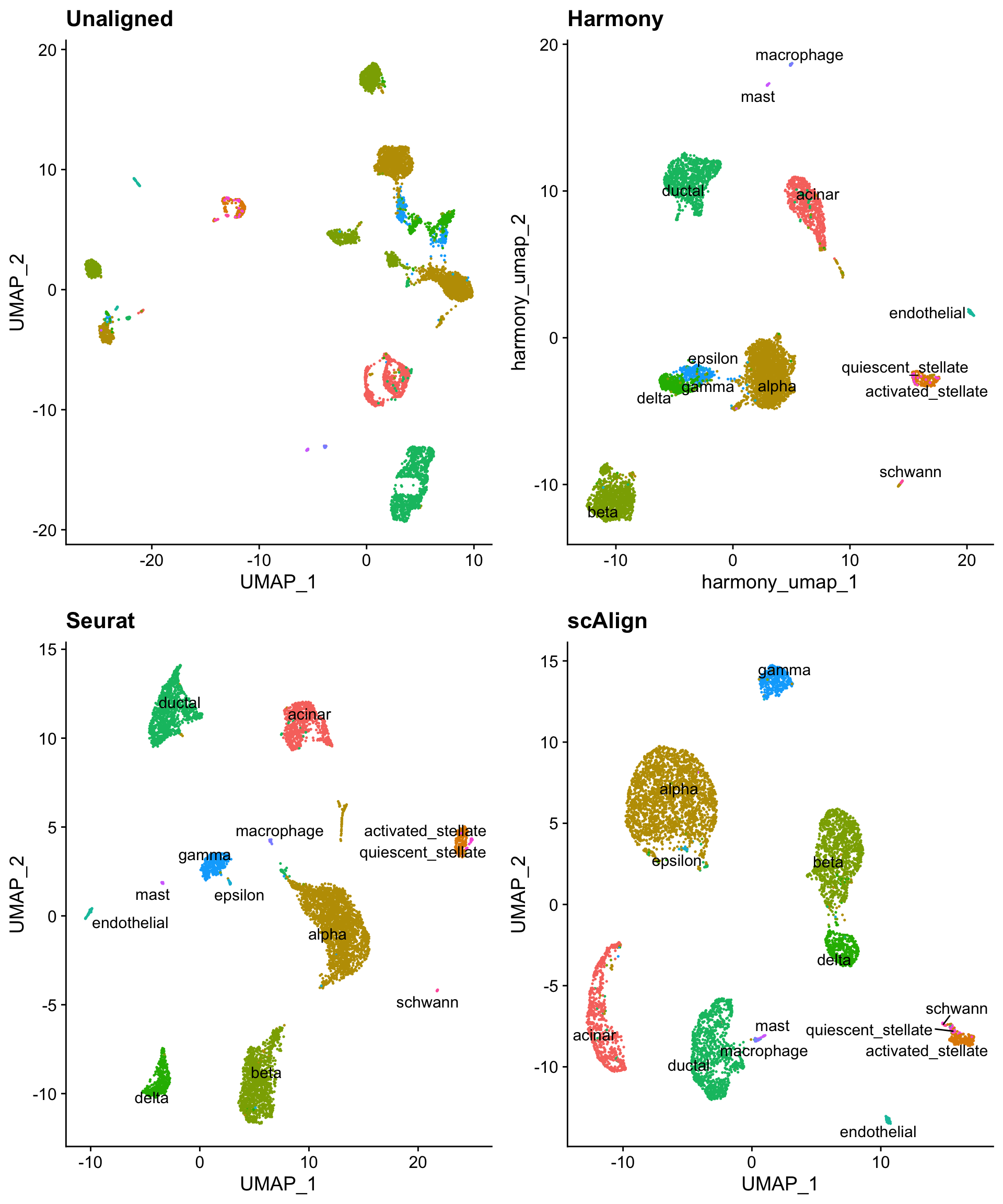
And all three techniques do a satisfactory job of eliminating intra-cluster technology bias.
CombinePlots(list(pre_tech_plot + ggtitle("Unaligned"),
                  h_umap_tech_plot + ggtitle("Harmony"),
                  s_umap_tech_plot + ggtitle("Seurat"),
                  sca_umap_tech_plot + ggtitle("scAlign")),
             legend = "none",
             ncol = 2)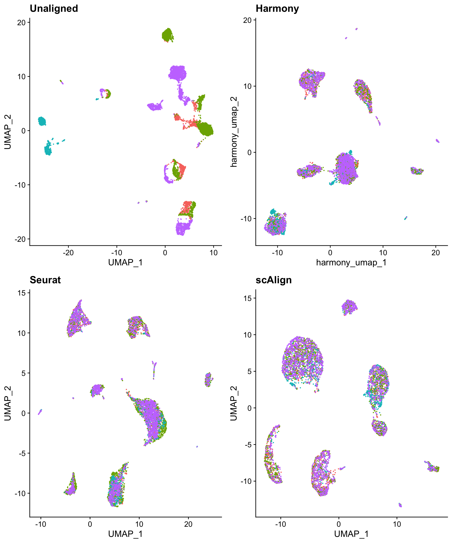
Ultimately, method selection, tuning, and assessment is highly dependent on knowledge of the experimental design and underlying biology.