The RMD file to follow along: https://scrnaseq-workshop.s3-us-west-2.amazonaws.com/4_markers.Rmd
finding markers and differential expression analysis
After clustering, differential expression testing (DE analysis, similar to bulk RNA seq) finds gene signatures of each cluster/cell population, to give more insights into biology.
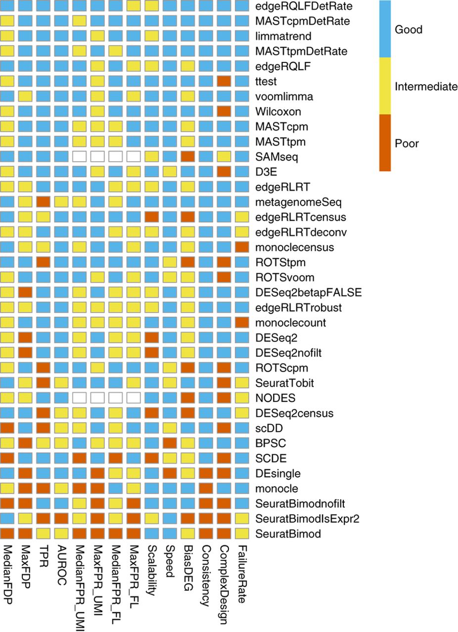
many proposed methods
(for Seurat, we recommend default “wilcox” or “t”, good balances between speed and accuracy)
important considerations
keep things simple first and look at the results (try not aligning, not regressing)
determine what variables to regress out (batch, nCount_RNA, percent_mito, cell cycle, if needed) during scaling (note this only affects dimension reduction and clustering)
library(Seurat)
library(tidyverse)
# load data from saved RDS
sobj <- readRDS("_vignettes/data/filtered_sobj.rds")

# log normalize
sobj_l <- NormalizeData(sobj) # <- skip this step if using scran normalization
sobj_l <- ScaleData(sobj_l,
                    vars.to.regress = c("nCount_RNA",
                                        "percent_mito"))

# alternatively, sctransform is a one step normalization and scaling process
sobj_sc <- suppressWarnings(SCTransform(object = sobj, # sctransform has some unhelpful warnings
                                        vars.to.regress = c("percent_mito"), # already corrects for transcript number
verbose = FALSE))- use normalized data for DE (slot is dependent on normalization method, also don’t use integrated assay)
# before normalization, "data" slot is the same as counts
sobj@assays$RNA@data[101:105,101:105] # raw counts
#> 5 x 5 sparse Matrix of class "dgCMatrix"
#>        ATCTTGACCTCCCA-1 ATCTTTCTTGTCCC-1 ATGAAGGACCTGTC-1
#> PGD                   2                .                .
#> APITD1                .                .                .
#> DFFA                  .                .                .
#> PEX14                 .                .                .
#> CASZ1                 .                .                .
#>        ATGACGTGATCGGT-1 ATGAGAGAAGTAGA-1
#> PGD                   .                .
#> APITD1                .                .
#> DFFA                  .                .
#> PEX14                 .                .
#> CASZ1                 .                .

# after log normalization, results are stored in "data" slot
sobj_l@assays$RNA@data[101:105,101:105] # normalized
#> 5 x 5 sparse Matrix of class "dgCMatrix"
#>        ATCTTGACCTCCCA-1 ATCTTTCTTGTCCC-1 ATGAAGGACCTGTC-1
#> PGD            2.727586                .                .
#> APITD1         .                       .                .
#> DFFA           .                       .                .
#> PEX14          .                       .                .
#> CASZ1          .                       .                .
#>        ATGACGTGATCGGT-1 ATGAGAGAAGTAGA-1
#> PGD                   .                .
#> APITD1                .                .
#> DFFA                  .                .
#> PEX14                 .                .
#> CASZ1                 .                .

# after sctransform, results are stored in new assay "SCT"
sobj_sc@assays$SCT@data[101:105,101:105] # normalized
#> 5 x 5 sparse Matrix of class "dgCMatrix"
#>        ATCTTGACCTCCCA-1 ATCTTTCTTGTCCC-1 ATGAAGGACCTGTC-1
#> PGD            1.386294                .                .
#> APITD1         .                       .                .
#> DFFA           .                       .                .
#> PEX14          .                       .                .
#> CASZ1          .                       .                .
#>        ATGACGTGATCGGT-1 ATGAGAGAAGTAGA-1
#> PGD                   .                .
#> APITD1                .                .
#> DFFA                  .                .
#> PEX14                 .                .
#> CASZ1                 .                .
sobj_sc@assays$RNA@data[101:105,101:105] # still same as counts, make sure not to use this!
#> 5 x 5 sparse Matrix of class "dgCMatrix"
#>        ATCTTGACCTCCCA-1 ATCTTTCTTGTCCC-1 ATGAAGGACCTGTC-1
#> PGD                   2                .                .
#> APITD1                .                .                .
#> DFFA                  .                .                .
#> PEX14                 .                .                .
#> CASZ1                 .                .                .
#>        ATGACGTGATCGGT-1 ATGAGAGAAGTAGA-1
#> PGD                   .                .
#> APITD1                .                .
#> DFFA                  .                .
#> PEX14                 .                .
#> CASZ1                 .                .
Note that marker genes found is very dependent on clustering and the compared populations
P‐values are inflated, due to the cyclic nature of identifying the same variable genes as markers, which were used for dimension reduction and clustering. However, the ranking of genes based on P‐values is unaffected.
Sidebar: How to regress out cell cycle heterogeneity (and do you need to?)
# many options to assess cell cycle effects on gene expression
# 1. ridge plot on key genes (from Seurat2 tutorial)
RidgePlot(sobj_l,
          features = c("MKI67", # smoothing eaves plots empty if no significant amount of cells express it
                       "MCM6",
                       "TOP2A",
                       "PCNA",
                       "ZFP36"), # how actual robust gene expression should look
          ncol = 2)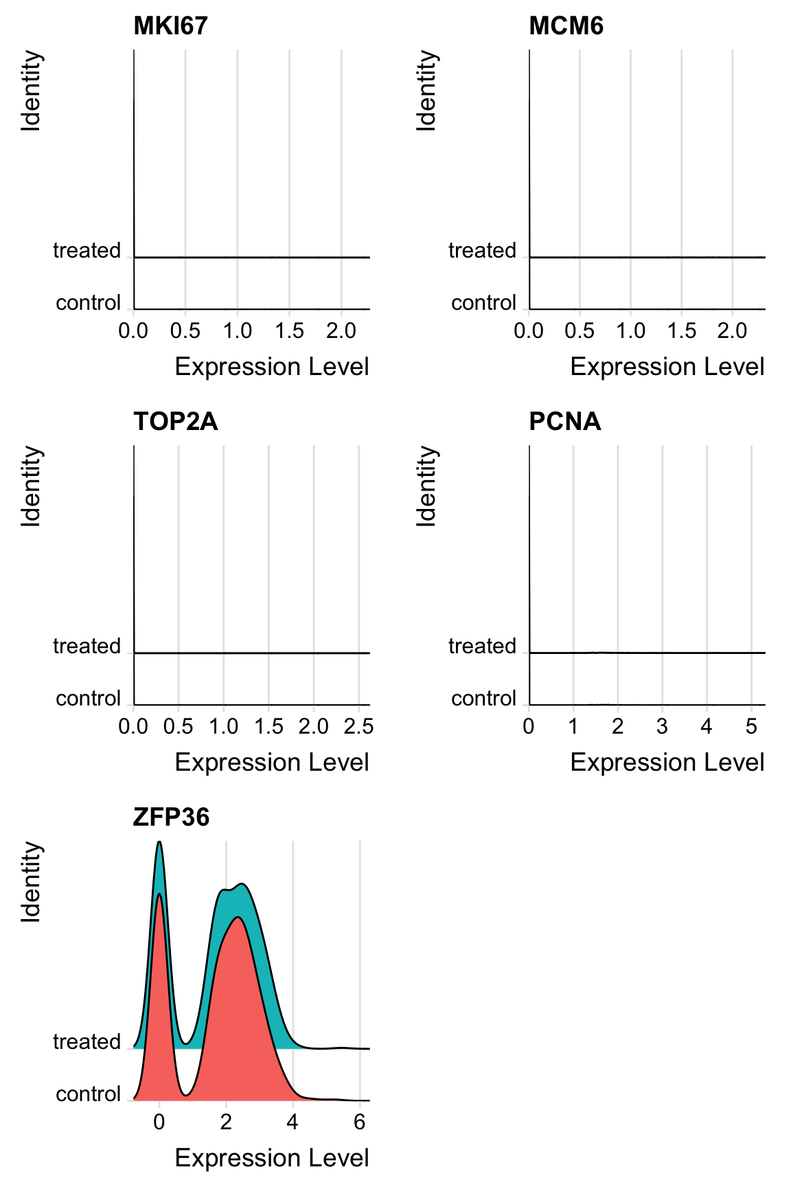
# see https://satijalab.org/seurat/v3.0/cell_cycle_vignette.html for a case where some cells are actively cycling
# 2. assess phase and PCA
# Seurat stores a list of cell cycle specific genes for humans
s.genes <- Seurat::cc.genes$s.genes # obviously unsuitable for nonhuman
g2m.genes <- Seurat::cc.genes$g2m.genes

s.genes
#>  [1] "MCM5"     "PCNA"     "TYMS"     "FEN1"     "MCM2"     "MCM4"
#>  [7] "RRM1"     "UNG"      "GINS2"    "MCM6"     "CDCA7"    "DTL"
#> [13] "PRIM1"    "UHRF1"    "MLF1IP"   "HELLS"    "RFC2"     "RPA2"
#> [19] "NASP"     "RAD51AP1" "GMNN"     "WDR76"    "SLBP"     "CCNE2"
#> [25] "UBR7"     "POLD3"    "MSH2"     "ATAD2"    "RAD51"    "RRM2"
#> [31] "CDC45"    "CDC6"     "EXO1"     "TIPIN"    "DSCC1"    "BLM"
#> [37] "CASP8AP2" "USP1"     "CLSPN"    "POLA1"    "CHAF1B"   "BRIP1"
#> [43] "E2F8"
g2m.genes
#>  [1] "HMGB2"   "CDK1"    "NUSAP1"  "UBE2C"   "BIRC5"   "TPX2"
#>  [7] "TOP2A"   "NDC80"   "CKS2"    "NUF2"    "CKS1B"   "MKI67"
#> [13] "TMPO"    "CENPF"   "TACC3"   "FAM64A"  "SMC4"    "CCNB2"
#> [19] "CKAP2L"  "CKAP2"   "AURKB"   "BUB1"    "KIF11"   "ANP32E"
#> [25] "TUBB4B"  "GTSE1"   "KIF20B"  "HJURP"   "CDCA3"   "HN1"
#> [31] "CDC20"   "TTK"     "CDC25C"  "KIF2C"   "RANGAP1" "NCAPD2"
#> [37] "DLGAP5"  "CDCA2"   "CDCA8"   "ECT2"    "KIF23"   "HMMR"
#> [43] "AURKA"   "PSRC1"   "ANLN"    "LBR"     "CKAP5"   "CENPE"
#> [49] "CTCF"    "NEK2"    "G2E3"    "GAS2L3"  "CBX5"    "CENPA"

# score and phase call is added to metadata
sobj_l <- CellCycleScoring(sobj_l,
                           s.features = s.genes,
                           g2m.features = g2m.genes,
                           set.ident = FALSE)
sobj_l@meta.data %>% head()
#>                  orig.ident nCount_RNA nFeature_RNA percent_mito
#> AAACATACAACCAC-1    control       2419          779     3.017776
#> AAACATTGAGCTAC-1    control       4901         1350     3.795144
#> AAACGCTGACCAGT-1    control       2174          781     3.817847
#> AAACGCTGGTTCTT-1    control       2259          789     3.098716
#> AAAGTTTGATCACG-1    control       1265          441     3.478261
#> AAATCATGACCACA-1    control       4125         1365     4.581818
#>                      S.Score   G2M.Score Phase
#> AAACATACAACCAC-1  0.10140023 -0.05909799     S
#> AAACATTGAGCTAC-1 -0.03669937 -0.05460303    G1
#> AAACGCTGACCAGT-1 -0.04334459 -0.04401501    G1
#> AAACGCTGGTTCTT-1 -0.02891103  0.01944167   G2M
#> AAAGTTTGATCACG-1  0.09548679 -0.07351012     S
#> AAATCATGACCACA-1 -0.06976057 -0.01901402    G1

# check PCA to see if cell cycle has strong effects
sobj_l <- FindVariableFeatures(sobj_l)
sobj_l <- RunPCA(sobj_l, verbose = FALSE, npcs = 10)
DimPlot(sobj_l, group.by = "Phase") # again, in this case, cell cycle does not have strong effects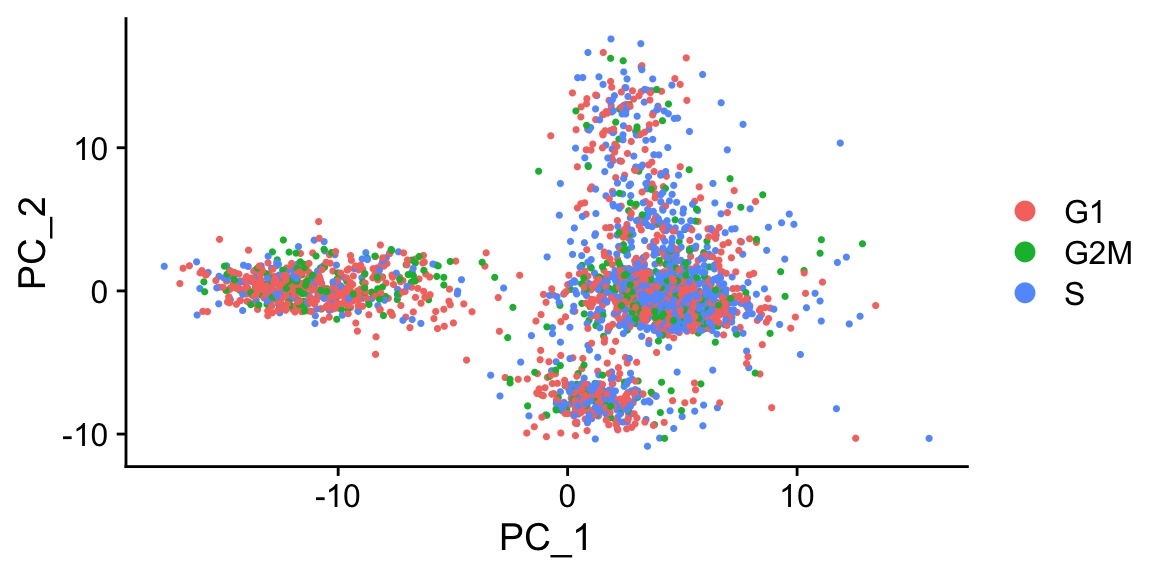
# 3. look for cell cycle-specific genes as main drivers of PCA
topPCAgenes <- apply(
  sobj_l@reductions$pca@feature.loadings, # contribution of each gene to each PC is stored here
  MARGIN = 2,
  FUN = function(x) names(sort(abs(x), decreasing = TRUE)[1:10]) # finds the most important genes in each PC
  )

topPCAgenes
#>       PC_1     PC_2     PC_3       PC_4        PC_5
#>  [1,] "CST3"   "NKG7"   "HLA-DQA1" "PF4"       "CKB"
#>  [2,] "S100A9" "CST7"   "CD79A"    "SDPR"      "FCGR3A"
#>  [3,] "TYROBP" "GZMA"   "CD79B"    "PPBP"      "MS4A7"
#>  [4,] "FTL"    "PRF1"   "HLA-DPB1" "HIST1H2AC" "RP11-290F20.3"
#>  [5,] "LST1"   "GZMB"   "CD74"     "GNG11"     "RHOC"
#>  [6,] "FCN1"   "FGFBP2" "HLA-DPA1" "SPARC"     "SIGLEC10"
#>  [7,] "AIF1"   "GNLY"   "MS4A1"    "GP9"       "LILRA3"
#>  [8,] "LYZ"    "CTSW"   "HLA-DQB1" "NRGN"      "LGALS2"
#>  [9,] "FTH1"   "CD79A"  "HLA-DRB1" "RGS18"     "HMOX1"
#> [10,] "S100A8" "CCL4"   "PPBP"     "PTCRA"     "MS4A6A"
#>       PC_6      PC_7      PC_8         PC_9       PC_10
#>  [1,] "GZMK"    "CCL5"    "FCER1A"     "IFIT1"    "IFIT1"
#>  [2,] "IL32"    "GZMK"    "CLEC10A"    "ISG15"    "ISG15"
#>  [3,] "GZMB"    "FCER1A"  "ENHO"       "MX1"      "ANXA1"
#>  [4,] "SPON2"   "KLRG1"   "SERPINF1"   "GZMK"     "PTTG1"
#>  [5,] "VIM"     "CLEC10A" "CD1C"       "IFI6"     "GBP1"
#>  [6,] "S100A4"  "SELL"    "GZMK"       "OASL"     "LTB"
#>  [7,] "AKR1C3"  "LYAR"    "RBP7"       "TNFSF10"  "MX1"
#>  [8,] "B2M"     "NKG7"    "CLIC2"      "ACTG1"    "PCNA"
#>  [9,] "S100A10" "AKR1C3"  "RP6-91H8.3" "APOBEC3B" "HOPX"
#> [10,] "S100B"   "IGFBP7"  "S100A12"    "LYAR"     "CD27"

topPCAgenes %>%
  as.vector() %>%
  intersect(c(s.genes, g2m.genes)) # see how many S and G2M genes intersect with that list
#> [1] "PCNA"

# or just check top variable genes
# if needed, regress out cell cycle effects
sobj_l <- ScaleData(sobj_l,
                    vars.to.regress = c("nCount_RNA", "percent_mito", "S.Score", "G2M.Score"))

# alternatively, leave the difference of cycling vs noncycling in place, only regress out phases in actively cycling cells
sobj_l$CC.Difference <- sobj_l$S.Score - sobj_l$G2M.Score
sobj_l <- ScaleData(sobj_l,
                    vars.to.regress = c("nCount_RNA",
                                        "percent_mito",
                                        "CC.Difference"))
find all markers for each cluster
FindAllMarkers compares cells in each cluster to all other cells in the dataset. Typically, focus is given to genes upregulated in each cluster, ie markers.
# load clustered object
sobj_clusters <- readRDS("_vignettes/data/clustered_sobj.rds")

# also check/set ident to the desired comparison
Idents(sobj_clusters) %>% head()
#> AAACATACAACCAC-1 AAACATTGAGCTAC-1 AAACGCTGACCAGT-1 AAACGCTGGTTCTT-1
#>                0                2                3                3
#> AAAGTTTGATCACG-1 AAATCATGACCACA-1
#>                2                5
#> Levels: 0 1 2 3 4 5 6 7
Idents(sobj_clusters) <- sobj_clusters@meta.data$clusters

markers_df <- FindAllMarkers(sobj_clusters,
                             assay = "RNA", # <- be careful with sobj_sc and intergrated objects
                             slot = "data",
                             only.pos = TRUE)
markers_df %>% head()
#>               p_val avg_logFC pct.1 pct.2     p_val_adj cluster  gene
#> LDHB  7.282957e-247 1.1811710 0.926 0.483 9.156134e-243       0  LDHB
#> RPS12 3.142126e-222 0.8524704 1.000 0.988 3.950281e-218       0 RPS12
#> RPS25 1.258715e-211 0.8660816 1.000 0.966 1.582456e-207       0 RPS25
#> CD3D  6.379927e-201 1.0471003 0.873 0.261 8.020845e-197       0  CD3D
#> RPS27 1.100287e-196 0.7788876 0.999 0.990 1.383281e-192       0 RPS27
#> RPS3  2.473657e-192 0.7175880 1.000 0.991 3.109882e-188       0  RPS3
find DE genes for specific cell groups
For more control in the comparisons, use FindMarkers. Positive average log (natural) fold change represents higher expression of the gene in cells of ident.1. pct1 and 2 are percent detected in each ident/population.
# DE analysis for 2 clusters
markers_df2 <- FindMarkers(sobj_clusters,
                           assay = "RNA",
                           slot = "data",
                           ident.1 = "1",
                           ident.2 = "2",
                           test.use = "t")
markers_df2 %>% head()
#>                p_val avg_logFC pct.1 pct.2     p_val_adj
#> LYZ     0.000000e+00  4.586764 1.000 0.426  0.000000e+00
#> TYROBP  0.000000e+00  3.544515 0.994 0.111  0.000000e+00
#> CST3    0.000000e+00  3.459219 0.992 0.185  0.000000e+00
#> LGALS1 7.140047e-315  3.066783 0.980 0.131 8.976467e-311
#> S100A4 1.217470e-300  3.278204 1.000 0.358 1.530603e-296
#> S100A9 7.302898e-282  4.927262 0.996 0.136 9.181203e-278
FindMarkers defaults to the current active ident. To use other value groups, set idents to the intended column, or use the group.by argument.
# compare control vs treated in only cluster 1
markers_df3 <- FindMarkers(sobj_clusters,
                           assay = "RNA",
                           slot = "data",
                           subset.ident = "1", # <- if needed, subset on current ident first, then switch idents
                           group.by = "orig.ident", # <- grouping cells by this metadata column
                           ident.1 = "control",
                           ident.2 = "treated")
For greater control, assign new idents or new columns in metadata, and customize DE analysis pairs.
# set new idents for more customized comparisons
Idents(sobj_clusters,
       WhichCells(object = sobj_clusters,
                  idents = "1",
                  expression = ZFP36 >= 1, # would usually do this for transgenes etc
                  slot = 'data')) <- 'ZFP36.pos'
Idents(sobj_clusters,
       WhichCells(object = sobj_clusters,
                  idents = "1",
                  expression = ZFP36 < 1,
                  slot = 'data')) <- 'ZFP36.neg'
Idents(sobj_clusters) %>% head() # note that with this method, some cell idents might not be changed
#> AAACATACAACCAC-1 AAACATTGAGCTAC-1 AAACGCTGACCAGT-1 AAACGCTGGTTCTT-1
#>                0                2                3                3
#> AAAGTTTGATCACG-1 AAATCATGACCACA-1
#>                2                5
#> Levels: ZFP36.neg ZFP36.pos 0 2 3 4 5 6 7

markers_df4 <- FindMarkers(sobj_clusters,
                           ident.1 = "ZFP36.pos",
                           ident.2 = "ZFP36.neg")

# or something like:
# Idents(sobj_clusters,
#        WhichCells(object = sobj_clusters,
#                   idents = "1",
#                   expression = sizeFactors >= 1, # would usually do this for transgenes etc
#                   slot = 'data')) <- 'cluster1_large'
Genes of interest can then be visualized as violin plots or feature plots.
Idents(sobj_clusters) <- sobj_clusters@meta.data$clusters # plots are grouped by active ident
VlnPlot(sobj_clusters, "LYZ")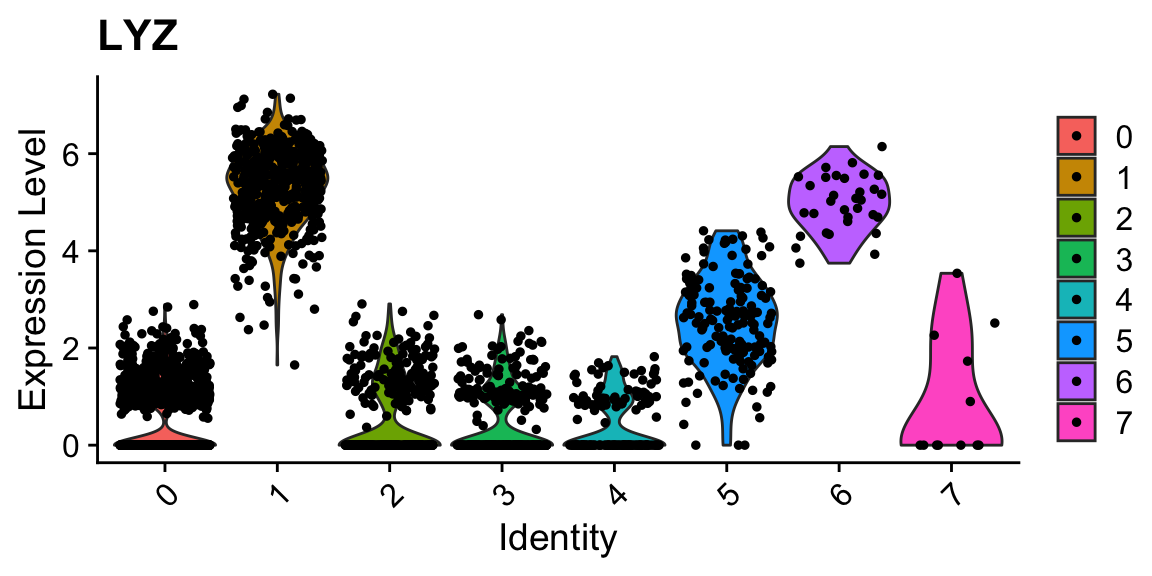
VlnPlot(sobj_clusters, c("ZFP36", "ZFP36L2")) # can be a vector of gene names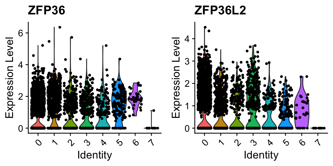
FeaturePlot(sobj_clusters, "LYZ")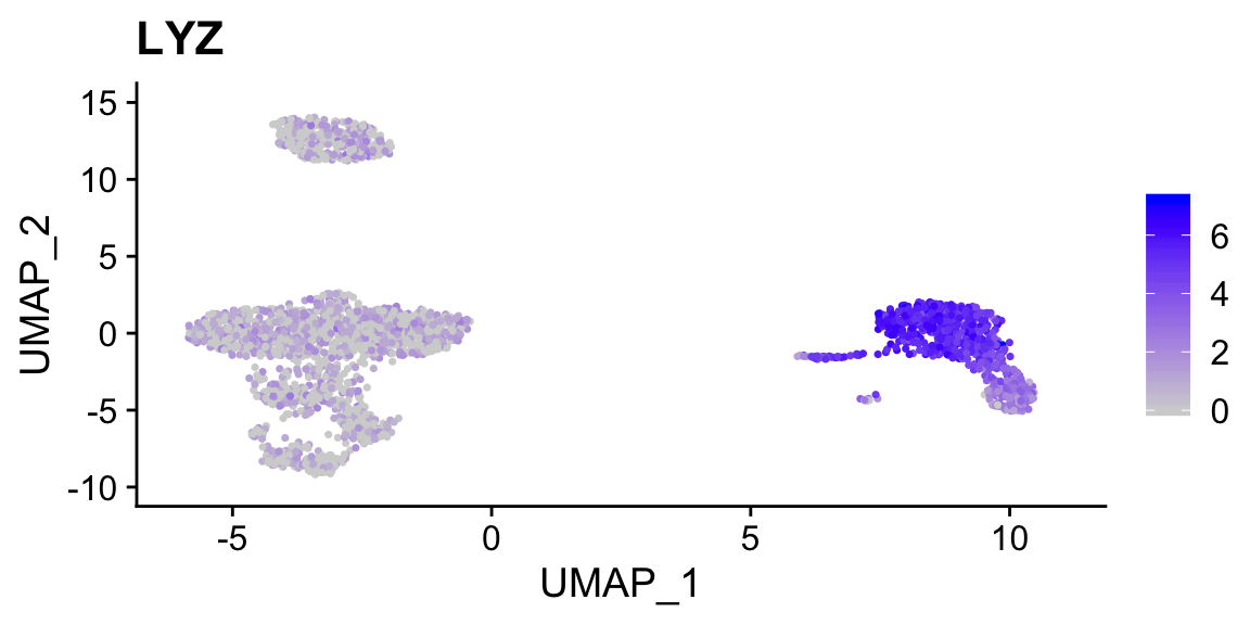
FeaturePlot(sobj_clusters, c("ZFP36", "ZFP36L2")) # can be a vector of gene names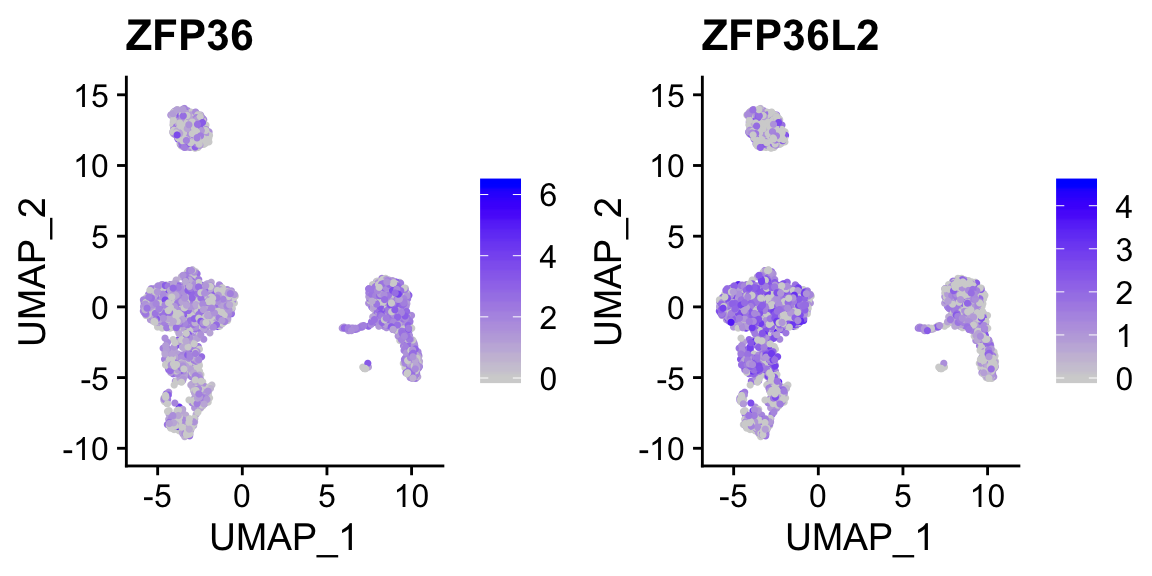
FeaturePlot(sobj_clusters, "ZFP36", split.by = "orig.ident") # <- split into panels based on metadata column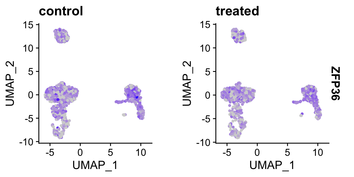
cluster identities
Without venturing into the realm of philosphical debates on what a “cell type” constitutes, standard pratice is to use certain gene expression features to classify cells. This is often done manually, by visual inspection of key genes. Automated approaches that utilize a broader range of features are currently being developed.
manual check and cluster identity assignment
# from the Seurat pancreas example
# we now have pan_celseq2, fully annotated in metadata column "celltype", and pan_smartseq2, ready to be annotated
data_url = "https://scrnaseq-workshop.s3-us-west-2.amazonaws.com"
pan_celseq2 <- readRDS(url(file.path(data_url, "pan_celseq2.rds")))
pan_celseq2@meta.data %>% head()
#>             orig.ident nCount_RNA nFeature_RNA    tech celltype
#> D28-1_1  SeuratProject  23438.618         5448 celseq2    alpha
#> D28-1_15 SeuratProject  27252.978         5918 celseq2    alpha
#> D28-1_17 SeuratProject  16177.715         4522 celseq2    alpha
#> D28-1_29 SeuratProject  39356.525         7416 celseq2    alpha
#> D28-1_30 SeuratProject  28958.986         6121 celseq2    alpha
#> D28-1_39 SeuratProject   7389.849         2746 celseq2    alpha
#>          RNA_snn_res.0.8 seurat_clusters
#> D28-1_1                8               8
#> D28-1_15               8               8
#> D28-1_17               0               0
#> D28-1_29               8               8
#> D28-1_30               8               8
#> D28-1_39               0               0
pan_smartseq2 <- readRDS(url(file.path(data_url, "pan_smartseq2.rds")))
pan_smartseq2@meta.data %>% head()
#>           orig.ident nCount_RNA nFeature_RNA      tech celltype
#> AZ_B9  SeuratProject     654549         4433 smartseq2    alpha
#> AZ_A6  SeuratProject     753413         4414 smartseq2    alpha
#> AZ_C1  SeuratProject    2044839         5069 smartseq2    alpha
#> AZ_A11 SeuratProject     705927         3900 smartseq2    alpha
#> AZ_C2  SeuratProject    1338503         5367 smartseq2    alpha
#> AZ_B11 SeuratProject    3378011         7137 smartseq2    alpha
#>        RNA_snn_res.0.8 seurat_clusters
#> AZ_B9               11              11
#> AZ_A6                7               7
#> AZ_C1               11              11
#> AZ_A11              11              11
#> AZ_C2               11              11
#> AZ_B11              11              11
a <- DimPlot(pan_smartseq2, label = TRUE) + NoLegend()
a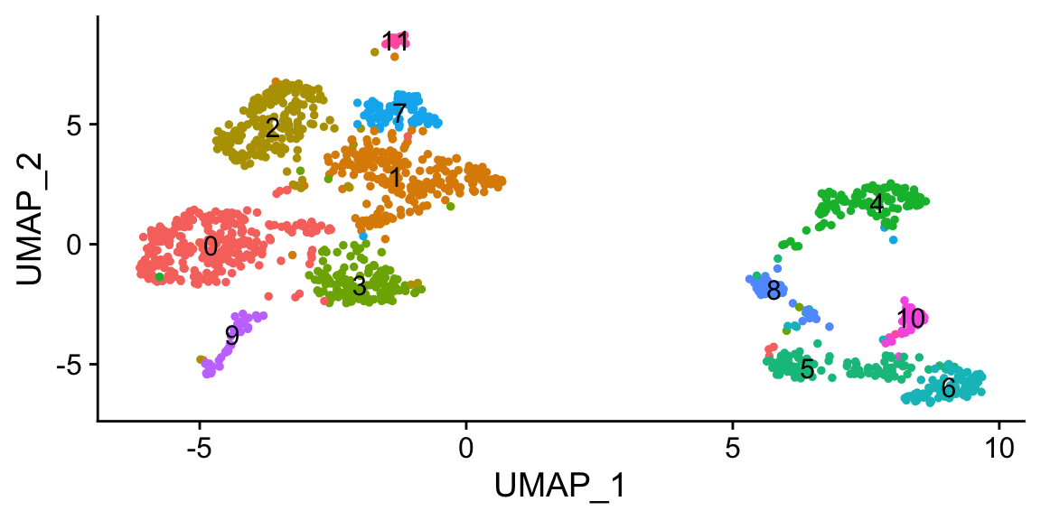
FeaturePlot(pan_smartseq2, c("IRX2","GC")) # marker genes for alpha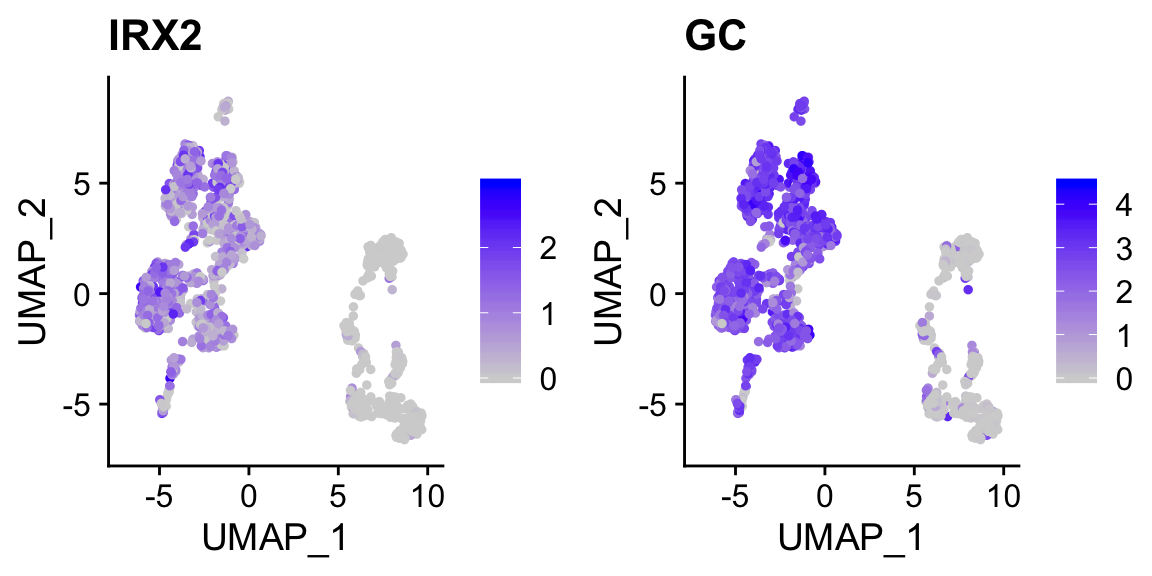
FeaturePlot(pan_smartseq2, c("IAPP","MAFA")) # marker genes for beta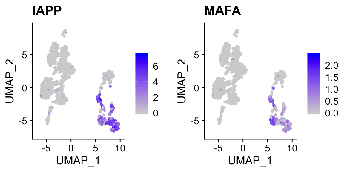
FeaturePlot(pan_smartseq2, c("HHEX","LEPR")) # marker genes for delta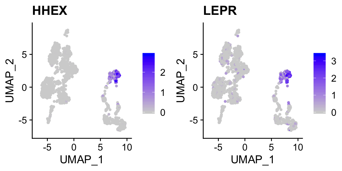
# optional, save the cluster numbers as "cluster.id"
pan_smartseq2 <- StashIdent(object = pan_smartseq2, save.name = "cluster.id") # or use AddMetaData

# Use RenameIdents to remap the idents from the current IDs to the new IDs
pan_smartseq2 <- RenameIdents(pan_smartseq2,
                              "0" = "alpha",
                              "1" = "alpha",
                              "2" = "alpha",
                              "3" = "alpha",
                              "7" = "alpha",
                              "9" = "alpha",
                              "11" = "alpha",
                              "5" = "beta",
                              "6" = "beta",
                              "8" = "beta",
                              "10" = "beta",
                              "4" = "delta")

# Plot UMAP with new cluster IDs
b <- DimPlot(object = pan_smartseq2,
        label = TRUE) + NoLegend()
b
cowplot::plot_grid(a,b)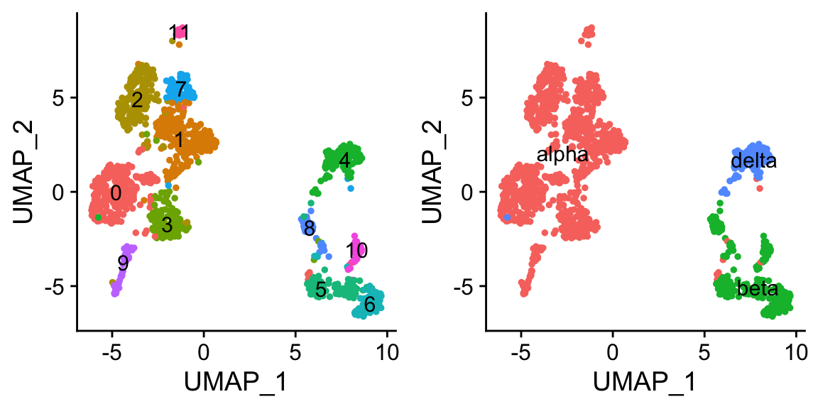
pan_smartseq2 <- StashIdent(object = pan_smartseq2, save.name = "cluster_name")
pan_smartseq2@meta.data %>% head()
#>           orig.ident nCount_RNA nFeature_RNA      tech celltype
#> AZ_B9  SeuratProject     654549         4433 smartseq2    alpha
#> AZ_A6  SeuratProject     753413         4414 smartseq2    alpha
#> AZ_C1  SeuratProject    2044839         5069 smartseq2    alpha
#> AZ_A11 SeuratProject     705927         3900 smartseq2    alpha
#> AZ_C2  SeuratProject    1338503         5367 smartseq2    alpha
#> AZ_B11 SeuratProject    3378011         7137 smartseq2    alpha
#>        RNA_snn_res.0.8 seurat_clusters cluster.id cluster_name
#> AZ_B9               11              11         11        alpha
#> AZ_A6                7               7          7        alpha
#> AZ_C1               11              11         11        alpha
#> AZ_A11              11              11         11        alpha
#> AZ_C2               11              11         11        alpha
#> AZ_B11              11              11         11        alpha
towards a more automated approach of identity assignment
- using
Seurat, inference from previous seurat object (requires very similar seurat object)
# reset idents of pan_smartseq2
Idents(pan_smartseq2) <- "cluster.id"

pancreas <- FindTransferAnchors(reference = pan_celseq2, query = pan_smartseq2,
    dims = 1:30)
predictions <- TransferData(anchorset = pancreas, refdata = pan_celseq2$celltype,
    dims = 1:30)
pan_smartseq2 <- AddMetaData(pan_smartseq2, metadata = predictions)
Idents(pan_smartseq2) <- "predicted.id"
DimPlot(pan_smartseq2, label = TRUE) + NoLegend()
- using
clustifyr, and marker gene list (requires markers or gene list), using gene list enrichment methods
# reset idents of pan_smartseq2
Idents(pan_smartseq2) <- "cluster.id"

# manually enter gene list
library(clustifyr)
beta <- c("IAPP","MAFA")
alpha <- c("IRX2","GC")
delta <- c("HHEX","LEPR")
genelist <- data.frame(alpha, beta, delta)
genelist
#>   alpha beta delta
#> 1  IRX2 IAPP  HHEX
#> 2    GC MAFA  LEPR

res <- clustify_lists(input = pan_smartseq2@assays$RNA@data,
                      marker = genelist,
                      cluster_info = pan_smartseq2@meta.data$seurat_clusters,
                      method = "jaccard") # calculate jaccard index

res # a matrix of scores
#>        alpha      beta   delta
#> 0  2.6714700 0.0000000 0.00000
#> 1  0.8017024 0.0000000 0.00000
#> 10 0.0000000 0.8017024 0.00000
#> 11 0.8017024 0.0000000 0.00000
#> 2  2.6714700 0.0000000 0.00000
#> 3  0.8017024 0.0000000 0.00000
#> 4  0.0000000 0.0000000 2.67147
#> 5  0.0000000 0.8017024 0.00000
#> 6  0.0000000 0.8017024 0.00000
#> 7  2.6714700 0.0000000 0.00000
#> 8  0.0000000 0.8017024 0.00000
#> 9  0.8017024 0.0000000 0.00000

res2 <- cor_to_call(res, threshold = 0.5) # take the highest, and if lower than cutoff, assign "unknown")
res2 # dataframe of identities
#> # A tibble: 12 x 3
#> # Groups:   cluster [12]
#>    cluster type      r
#>    <chr>   <chr> <dbl>
#>  1 0       alpha 2.67
#>  2 1       alpha 0.802
#>  3 11      alpha 0.802
#>  4 2       alpha 2.67
#>  5 3       alpha 0.802
#>  6 7       alpha 2.67
#>  7 9       alpha 0.802
#>  8 10      beta  0.802
#>  9 5       beta  0.802
#> 10 6       beta  0.802
#> 11 8       beta  0.802
#> 12 4       delta 2.67

namedres <- structure(res2$type, names = res2$cluster) # make named vector
namedres
#>       0       1      11       2       3       7       9      10
#> "alpha" "alpha" "alpha" "alpha" "alpha" "alpha" "alpha"  "beta"
#>       5       6       8       4
#>  "beta"  "beta"  "beta" "delta"

# seurat idents are factors, which may have strange behavior if coerced to numbers/index
namedres[as.character(Idents(pan_smartseq2))][1:10]
#>      11       7      11      11      11      11      11      11
#> "alpha" "alpha" "alpha" "alpha" "alpha" "alpha" "alpha" "alpha"
#>      11      11
#> "alpha" "alpha"
pan_smartseq2@meta.data$celltype <- namedres[as.character(Idents(pan_smartseq2))]
DimPlot(pan_smartseq2, label = T, group.by = "celltype") + NoLegend()
- using
clustifyr, and transcriptome profiles (from other scRNAseq, bulk RNAseq, or microarray), using ranked correlation of highly variable genes (scmap is another similar package)
# build a reference from expression matrix data
ref <- average_clusters(mat = pan_celseq2@assays$RNA@data,
                        cluster_info = pan_celseq2@meta.data,
                        cluster_col = "celltype")

res <- clustify(input = pan_smartseq2@assays$RNA@data,
                ref_mat = ref,
                metadata = pan_smartseq2@meta.data,
                query_genes = pan_smartseq2@assays$RNA@var.features, # using Seurat computed variable genes
                cluster_col = "seurat_clusters")
res2 <- cor_to_call(res, threshold = 0.5) # anything below 0.5 correlation are labeled as "unknown"
res2
#> # A tibble: 12 x 3
#> # Groups:   cluster [12]
#>    cluster type      r
#>    <chr>   <chr> <dbl>
#>  1 0       alpha 0.740
#>  2 1       alpha 0.716
#>  3 11      alpha 0.673
#>  4 2       alpha 0.755
#>  5 3       alpha 0.739
#>  6 7       alpha 0.731
#>  7 9       alpha 0.741
#>  8 10      beta  0.726
#>  9 5       beta  0.787
#> 10 6       beta  0.805
#> 11 8       beta  0.787
#> 12 4       delta 0.801

# same as last section
namedres <- structure(res2$type, names = res2$cluster)
pan_smartseq2@meta.data$celltype <- namedres[as.character(Idents(pan_smartseq2))]
DimPlot(pan_smartseq2, label = T, group.by = "celltype") + NoLegend()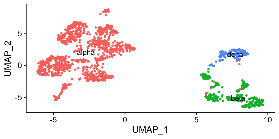
clustifyr also takes seurat objects as input directly, finds various needed data, and output another object with identities assigned.
ref <- seurat_ref(pan_celseq2,
                  cluster_col = "celltype")

res <- clustify(input = pan_smartseq2,
                ref_mat = ref,
                cluster_col = "seurat_clusters",
                seurat_out = TRUE)

res
#> An object of class Seurat
#> 34363 features across 1443 samples within 1 assay
#> Active assay: RNA (34363 features)
#>  2 dimensional reductions calculated: pca, umap

# look at UMAP
DimPlot(res, label = TRUE, group.by = "type") + NoLegend() # saved in "type" metadata column
Also see more tutorials at clustifyr, and prebuilt references from large scRNAseq/bulk RNAseq/microarray datasets at package clustifyrdata.
cell type composition
Insight into different samples can be gained from the proportion of cells that fall into each cell type. Unfortunately, no dedicated tools are available for statistical testing.
tab1 <- sobj_clusters@meta.data %>% group_by(orig.ident, clusters) %>% tally() # counting up all combinations
tab1
#> # A tibble: 16 x 3
#> # Groups:   orig.ident [2]
#>    orig.ident clusters     n
#>    <fct>      <fct>    <int>
#>  1 control    0          553
#>  2 control    1          243
#>  3 control    2          176
#>  4 control    3          190
#>  5 control    4           74
#>  6 control    5           80
#>  7 control    6           14
#>  8 control    7            6
#>  9 treated    0          589
#> 10 treated    1          250
#> 11 treated    2          176
#> 12 treated    3          150
#> 13 treated    4           87
#> 14 treated    5           78
#> 15 treated    6           18
#> 16 treated    7            6
tab2 <- tab1 %>% spread(key = clusters, value = n) # spread out into "wide" form
tab2
#> # A tibble: 2 x 9
#> # Groups:   orig.ident [2]
#>   orig.ident   `0`   `1`   `2`   `3`   `4`   `5`   `6`   `7`
#>   <fct>      <int> <int> <int> <int> <int> <int> <int> <int>
#> 1 control      553   243   176   190    74    80    14     6
#> 2 treated      589   250   176   150    87    78    18     6
tab3 <- tab1 %>% group_by(orig.ident) %>%
  mutate(n = n/sum(n)) %>% # convert counts to proportions first
  spread(key = clusters, value = n)
tab3
#> # A tibble: 2 x 9
#> # Groups:   orig.ident [2]
#>   orig.ident   `0`   `1`   `2`   `3`    `4`    `5`    `6`     `7`
#>   <fct>      <dbl> <dbl> <dbl> <dbl>  <dbl>  <dbl>  <dbl>   <dbl>
#> 1 control    0.414 0.182 0.132 0.142 0.0554 0.0599 0.0105 0.00449
#> 2 treated    0.435 0.185 0.130 0.111 0.0643 0.0576 0.0133 0.00443
and save tables to disk with write_csv
write_csv(tab3, "data/perc_clusters.csv")
tab4 <- read_csv("data/perc_clusters.csv")
other things to do with marker genes
gene list to pathway activity score, via
AUCellif TF expression is too low, consider
SCENICfor TF activity inferencestandard GO term enrichment tools
gProfiler2,enrichR,fgsea, etc etc