Single-cell RNA-seq Workshop: <b style="font-size:45px;">Introduction to scRNA-seq Analysis</b>

intro to RBI

rbi.fellows@ucdenver.edu,

RC1 South room9101

office hours on Thursday afternoons

outline of the workshop

Prereq: check all required packages are installed
Day 1 (pm):
- Say Hi
- Intro to scRNAseq
- Data preprocessing
- Import into R
- Quality control
Day 2 (am):
- Projections
- Clustering
- Finding markers
- Annotating cell types
Day 2 (pm):
- Pseudotime analysis
- Dataset alignment
Day 3 (am):
- Multimodal data (CITE-seq, hashing)
- Miscellaneous
Day 3 (pm) : working through your own data
Survey after the workshop for feedback

limitations of scRNAseq

dropout effect, only a small portion of the mRNAs from each cell is captured (see: GFP and other supposed markers)
low number of detectable genes, might not detect low expressing genes at all (see: TFs)
little info outside of gene counts (see: no tail-seq, isoform info)
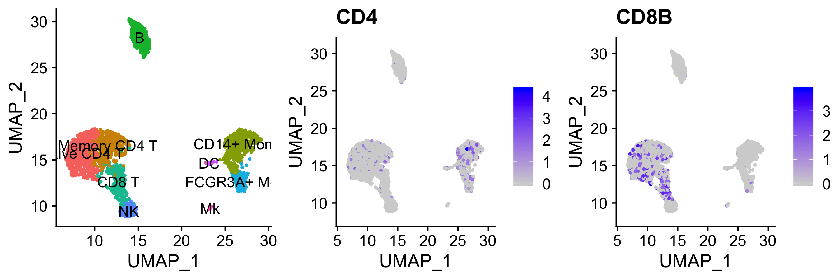
discrepancies between RNA and protein, especially surface proteins (see: CD4+ vs CD8+)
constantly evolving chemistry and bioinformatics tools (see: 10x v2/v3/v3.1, bad cell calling in cellrangerV2)

experimental design >> informatics corrections

too few or too many cells - 1000 cell lower limit for capture, and waste of money
doublets - 10000 cells ~ 10% doublet rate
(try: scrublet)
cell death - worse RNA capture, potentially different expression profile
(try: MT-RNA cutoff, regress out MT-RNA score)
lysed/free RNA - background for all cells, interferes with clustering and markers
(try: SoupX)

different sex of mice in samples - makes sample comparisons harder
(try: ignore known sex-dependent genes)
batch effects - still preferable to have all, or at least the direct comparison samples, captured at the same time
(try: various alignment methods)
n = ? - no consensus in the field, but aggregating 2 or more biological repeats, or hash multiple samples at the same time, should be valid

single cell RNA sequencing overview

cell suspension -> cDNA library -> fastq file -> gene expression matrix ->

filtering -> preprocessing -> dimension reduction -> clustering -> identity and markers -> pseudotime

1. sequencing methods

main platforms: 10x vs Smart-seq2 vs sci-RNA-seq3

method	cell isolation	coverage	saturation read #	gene detection	throughput and cost
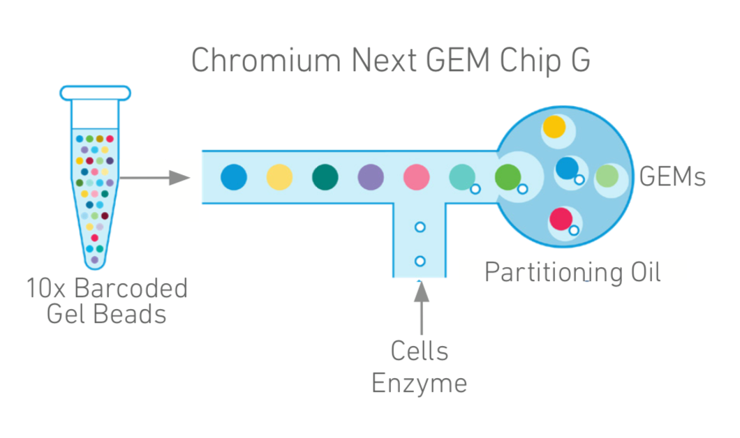
10x Chromium	droplet-based	polyA+ 3’ only	10^5 per cell	~2000 per cell	~5k cells, low cost
Smart-seq2	FACS-sorted	full length	10^6 per cell	~4000 per cell	manual pipetting, high cost
sci-RNA-seq3	combinatorial index	polyA+ 3’ only	10^5 per cell	~1000 per cell	~1m cells, lowest cost per

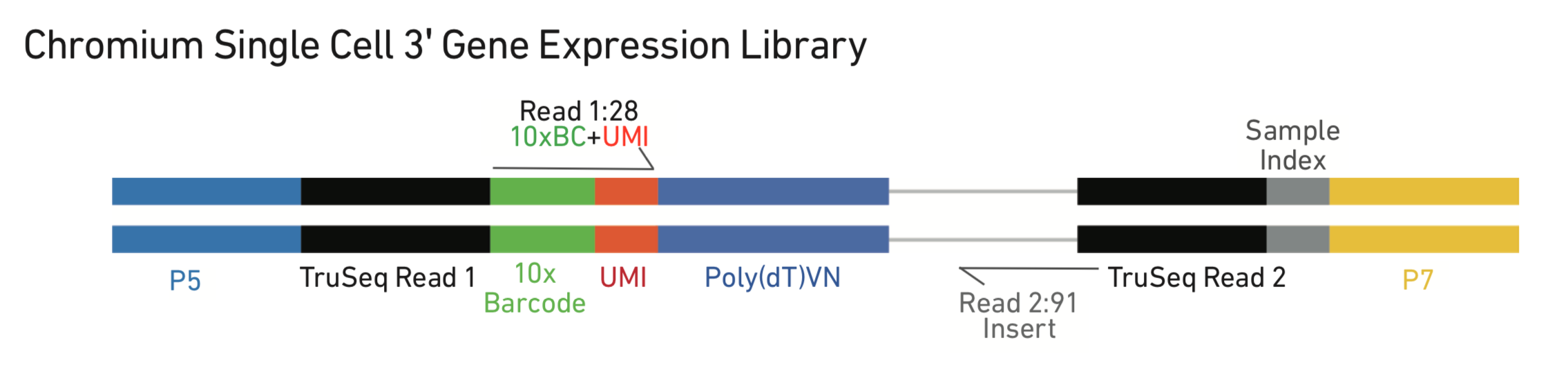
variations within 10x system: standard 3’, 5’ + V(D)J, antibody hashing, CITE-seq, variant-calling (very different sample preps, may require up to 4 library preps per sample)

2. alignment pipelines

cellranger performs alignment, filtering, UMI counting, clustering, and gene expression analysis.

Alternatives such as Alevin, STARsolo, Kallisto


# in terminal
cellranger count --id=123 \ 
                 --transcriptome=/refdata-cellranger-GRCh38-3.0.0 \ 
                 # build new transcriptome if you have GFP/RFP/transgene
                 --fastqs=/home/runs/HAT7ADXX/outs/fastq_path \ 
                 # a list of fastqs, a folder, or pass table via csv file
                 --sample=mysample 
                 # will need additional arguments for feature barcoding

output folder structure


KO_1_CDNA
|-- KO_1_CDNA.mri.tgz
|-- SC_RNA_COUNTER_CS
|   |-- CLOUPE_PREPROCESS
|   |-- EXPAND_SAMPLE_DEF
|   |-- SC_RNA_COUNTER
|   `-- fork0
|-- _cmdline
|-- _filelist
|-- _finalstate
|-- _invocation
|-- _jobmode
|-- _log
|-- _mrosource
|-- _perf
|-- _sitecheck
|-- _tags
|-- _timestamp
|-- _uuid
|-- _vdrkill
|-- _versions
`-- outs
    |-- analysis
    |-- cloupe.cloupe # cloupe file for browser view
    |-- filtered_feature_bc_matrix # use this fold for seurat
    |-- filtered_feature_bc_matrix.h5
    |-- metrics_summary.csv
    |-- molecule_info.h5
    |-- possorted_genome_bam.bam
    |-- possorted_genome_bam.bam.bai
    |-- raw_feature_bc_matrix # or this for seurat
    |-- raw_feature_bc_matrix.h5
    `-- web_summary.html # qc summary

~ 5-8 hours per sample on biochem department cluster “Bodhi”

theoretically can be ran locally on linux, but will require at least 32GB of RAM

other campus options include Rosalind, AWS

cellranger output html and loupe files

3. key things to check for in the initial output html report

number of cells close to expectations? reasonable elbow plot?
reads per cell (this is merely calculated as reads/cells, so somewhat inaccurate) - ideally ~50-100k
genes per cell, ideally ~2000
sequencing saturation?
any structure in the dimension reduction tSNE?

4. downstream processing in R or python

more accurate cell calling
more stringent filtering
regress out unwanted sources of variance
appropriate choice of normalization method
UMAP instead of tSNE projections, and fine-tuning
fine-tuning of dataset alignment methods and parameters (by default cellranger does align during aggregation)
find marker genes and assign cluster identities (may merge some)
more flexible visualizations
GO term analysis and other things
export to a hosted browser, similar to cloupe

reading and making UMI-barcode elbow plots

The total UMI (unique molecular identifier - represent each transcript) of a cell barcode is used to rank the barcodes determine the UMI threshold for signal vs noise. A plot is generated for cellranger html output, but will also be useful in other situations like hashing and CITE-seq.

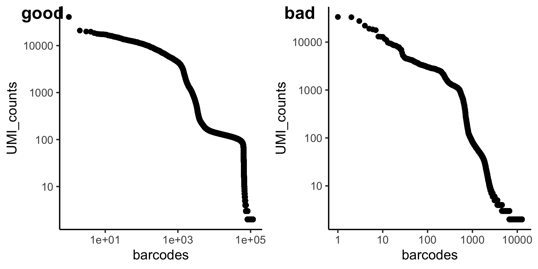
for a standard 10x scRNAseq run:

expected range of x axis (barcode) : ~ 10^5 (if using ggplot to visualize, filter)

expected inflection point of x axis (cell number): ~ # of loaded cells / 2

expected range of y axis (UMI_counts) : ~ 10^4

expected inflection point of y axis (cutoff UMI count): ~ 1000


library(tidyverse)
# use "raw" instead of "filtered" cellranger output folder
data_url = "https://scrnaseq-workshop.s3-us-west-2.amazonaws.com"
m1 <- readRDS(url(file.path(data_url, "raw_matrix.rds")))
# all genes x all barcodes

counts <- Matrix::colSums(m1) # calculate total UMI read number for each cell barcode
countdf <- as.data.frame(counts) %>% 
  as_tibble(rownames = "barcode") %>% 
  filter(counts >= 2) %>% # throw out cell barcodes with 1 or less UMI, this is mainly for time purposes
  arrange(desc(counts)) %>% # arrange by descending order
  mutate(rank = 1:n()) # rank

head(countdf) # barcodes now ranked by UMI counts
#> # A tibble: 6 x 3
#>   barcode          counts  rank
#>   <chr>             <dbl> <int>
#> 1 GCAGCCACATACCGTA  40745     1
#> 2 ATGGAGGGTGGTAACG  20916     2
#> 3 GTAACCATCGCTTGAA  19958     3
#> 4 TTCATGTGTCGTGTTA  19765     4
#> 5 GAATAGACATCCTGTC  18494     5
#> 6 GTCTCACGTTGGCCGT  17828     6

ggplot(countdf, aes(x = rank, y = counts)) +
  geom_point() +
  labs(x = "barcodes", y = "UMI_counts") +
  theme_classic() +
  scale_x_log10() + 
  scale_y_log10()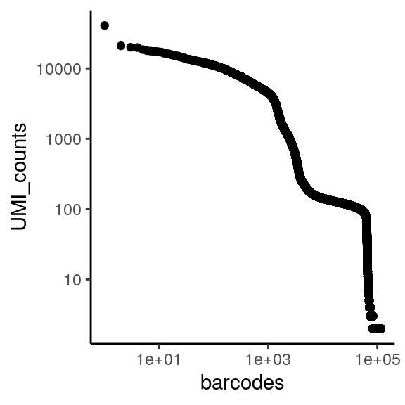

briefly, tidyverse/dplyr verbs

The tidyverse is a collection of R packages designed for data science. All packages share design philosophy, grammar, and data structures.

Seurat also uses some of the grammar, such as group.by.

A large amount of code introduced in this workshop in based on matrix and dataframe manipulation. Therefore some basic understanding of tidyverse/dplyr will be helpful.

Also, “%>%” is used as “pipe”, similar to unix |.


# we will look at metadata from pbmc_small from Seurat
library(Seurat)
library(tidyverse)
# note that tidyverse is philosophically against rownames

meta <- pbmc_small@meta.data %>% as_tibble(rownames = "cell_id")
meta %>% head() %>% print() # <- same as print(head(meta))
#> # A tibble: 6 x 8
#>   cell_id orig.ident nCount_RNA nFeature_RNA RNA_snn_res.0.8
#>   <chr>   <fct>           <dbl>        <int> <fct>          
#> 1 ATGCCA… SeuratPro…         70           47 0              
#> 2 CATGGC… SeuratPro…         85           52 0              
#> 3 GAACCT… SeuratPro…         87           50 1              
#> 4 TGACTG… SeuratPro…        127           56 0              
#> 5 AGTCAG… SeuratPro…        173           53 0              
#> 6 TCTGAT… SeuratPro…         70           48 0              
#> # … with 3 more variables: letter.idents <fct>, groups <chr>,
#> #   RNA_snn_res.1 <fct>


# "select" certain columns of data
meta2 <- meta %>% select(cell_id, 
                         nCount_RNA, 
                         RNA_snn_res.0.8, 
                         letter.idents)
meta2 %>% head() %>% print()
#> # A tibble: 6 x 4
#>   cell_id        nCount_RNA RNA_snn_res.0.8 letter.idents
#>   <chr>               <dbl> <fct>           <fct>        
#> 1 ATGCCAGAACGACT         70 0               A            
#> 2 CATGGCCTGTGCAT         85 0               A            
#> 3 GAACCTGATGAACC         87 1               B            
#> 4 TGACTGGATTCTCA        127 0               A            
#> 5 AGTCAGACTGCACA        173 0               A            
#> 6 TCTGATACACGTGT         70 0               A


# "filter" data to select specific rows
meta2 %>% filter(nCount_RNA >= 71, 
                 letter.idents == "A") %>%
  head() %>%
  print()
#> # A tibble: 6 x 4
#>   cell_id        nCount_RNA RNA_snn_res.0.8 letter.idents
#>   <chr>               <dbl> <fct>           <fct>        
#> 1 CATGGCCTGTGCAT         85 0               A            
#> 2 TGACTGGATTCTCA        127 0               A            
#> 3 AGTCAGACTGCACA        173 0               A            
#> 4 GCAGCTCTGTTTCT         72 0               A            
#> 5 AATGTTGACAGTCA        100 0               A            
#> 6 AGAGATGATCTCGC        191 0               A


# "arrange" the rows of your data into an order
meta2 %>% arrange(nCount_RNA) %>%
  head() %>%
  print()
#> # A tibble: 6 x 4
#>   cell_id        nCount_RNA RNA_snn_res.0.8 letter.idents
#>   <chr>               <dbl> <fct>           <fct>        
#> 1 CTTCATGACCGAAT         41 0               A            
#> 2 CATGAGACACGGGA         51 0               A            
#> 3 GATATAACACGCAT         52 0               A            
#> 4 AGGTCATGAGTGTC         62 0               A            
#> 5 TGGTATCTAAACAG         64 0               A            
#> 6 GTAAGCACTCATTC         67 0               A


# "mutate" your data frame to contain new columns
meta3 <- meta2 %>% mutate(seurat_clusters = str_c("cluster_", letter.idents), 
                          nCount_RNA_norm = nCount_RNA/max(nCount_RNA))
meta3 %>% head() %>% print()
#> # A tibble: 6 x 6
#>   cell_id nCount_RNA RNA_snn_res.0.8 letter.idents seurat_clusters
#>   <chr>        <dbl> <fct>           <fct>         <chr>          
#> 1 ATGCCA…         70 0               A             cluster_A      
#> 2 CATGGC…         85 0               A             cluster_A      
#> 3 GAACCT…         87 1               B             cluster_B      
#> 4 TGACTG…        127 0               A             cluster_A      
#> 5 AGTCAG…        173 0               A             cluster_A      
#> 6 TCTGAT…         70 0               A             cluster_A      
#> # … with 1 more variable: nCount_RNA_norm <dbl>


# "summarise" chunks of you data (by group) in some way.
meta3 %>% group_by(seurat_clusters) %>%
  summarise(n = n())
#> # A tibble: 2 x 2
#>   seurat_clusters     n
#>   <chr>           <int>
#> 1 cluster_A          53
#> 2 cluster_B          27

Introduction to scRNA-seq Analysis