This vignette provides detailed examples for plotting V(D)J data imported into a single-cell object using djvdj. For the examples shown below, we use data for splenocytes from BL6 and MD4 mice collected using the 10X Genomics scRNA-seq platform. MD4 B cells are monoclonal and specifically bind hen egg lysozyme.
library(djvdj)
library(Seurat)
library(ggplot2)

# Load GEX data
data_dir <- system.file("extdata/splen", package = "djvdj")

gex_dirs <- c(
  BL6 = file.path(data_dir, "BL6_GEX/filtered_feature_bc_matrix"),
  MD4 = file.path(data_dir, "MD4_GEX/filtered_feature_bc_matrix")
)

so <- gex_dirs |>
  Read10X() |>
  CreateSeuratObject() |>
  AddMetaData(splen_meta)

# Add V(D)J data to object
vdj_dirs <- c(
  BL6 = system.file("extdata/splen/BL6_BCR", package = "djvdj"),
  MD4 = system.file("extdata/splen/MD4_BCR", package = "djvdj")
)

so <- so |>
  import_vdj(
    vdj_dirs,
    define_clonotypes = "cdr3_gene",
    include_mutations = TRUE
  )
Histograms
The plot_histogram() function can be used to plot
numerical V(D)J data present in the object. By default, this will plot
the values present in the data_col column for every cell.
If data_col contains per-chain data (i.e. the column
contains the character specified by sep, default is ‘;’),
the values will be summarized for each cell. By default the mean will be
calculated. Cells that lack V(D)J data are removed before plotting, so
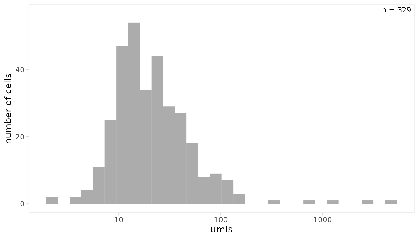
for this example we have 329 cells with V(D)J data. The
trans argument can be used to specify an x-axis
transformation.
In the example below, the mean number of UMIs per cell is plotted.
so |>
  plot_histogram(
    data_col = "umis",
    trans    = "log10"
  )
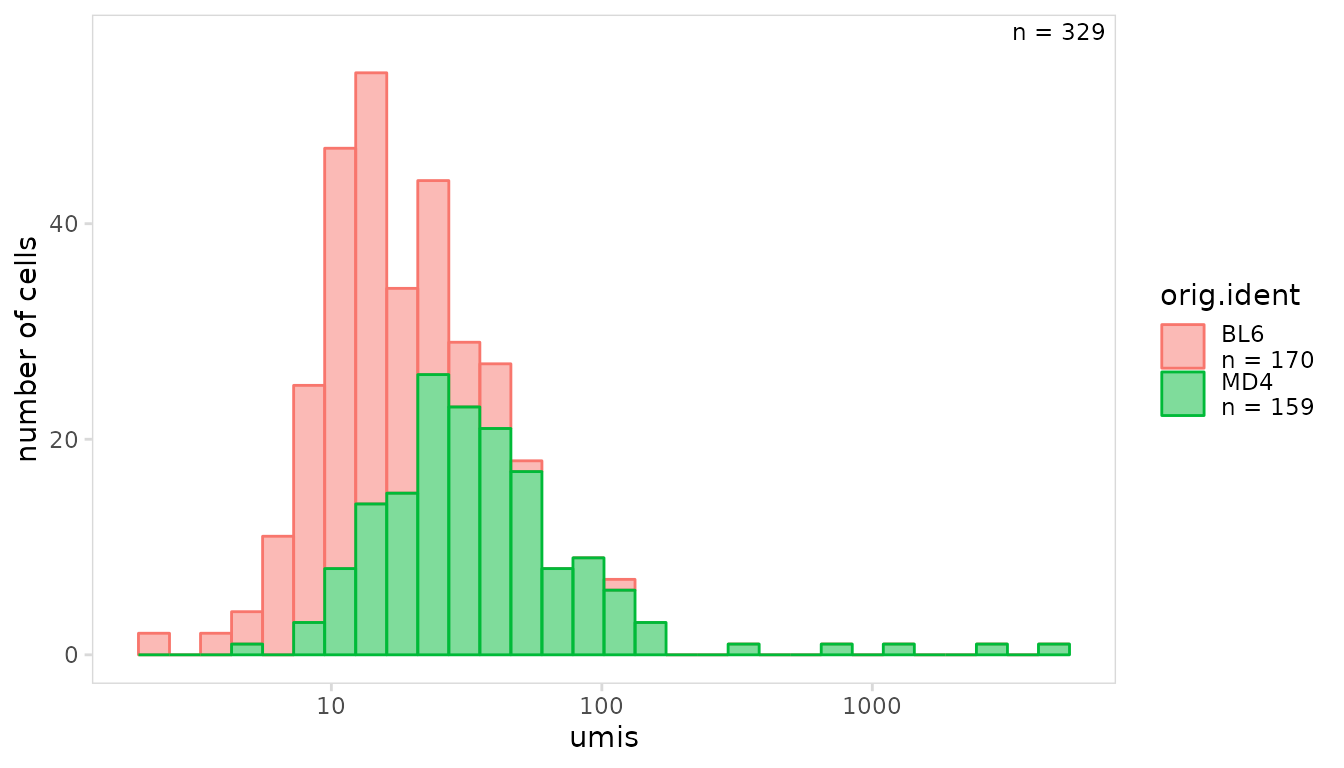
To color cells based on an additional variable present in the object,
specify the column name to the cluster_col argument.
so |>
  plot_histogram(
    data_col    = "umis",
    cluster_col = "orig.ident",
    trans       = "log10"
  )
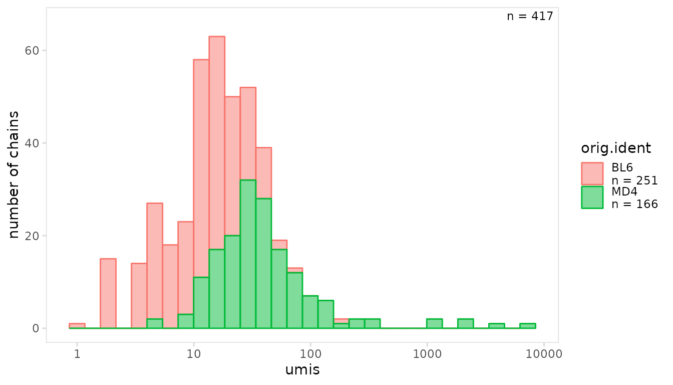
The function used to summarize per-chain values can be changed using
the summary_fn argument. The per-chain values can also be
plotted separately using the per_chain argument.
In the example below, the value for each chain is plotted.
so |>
  plot_histogram(
    data_col    = "umis",
    cluster_col = "orig.ident",
    per_chain   = TRUE,
    trans       = "log10"
  )
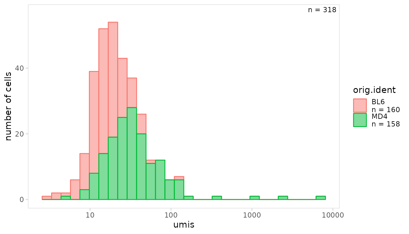
To only plot values for a specific chain, the chain
argument can be used. In this example the mean number of UMIs is shown
for each IGK chain.
so |>
  plot_histogram(
    data_col    = "umis",
    cluster_col = "orig.ident",
    chain       = "IGK",
    trans       = "log10"
  )
Violin plots
The plot_violin() function has similar functionality as
plot_histogram() but will generate violin plots or
boxplots. For all djvdj plotting functions additional arguments can be
passed directly to ggplot2 to further modify plot aesthetics. By default
clusters are arranged highest to lowest based on the values in
data_col. This ordering can be modified using the
plot_lvls argument”
vln <- so |>
  plot_violin(
    data_col    = "nCount_RNA",
    cluster_col = "sample",
    trans       = "log10",

    draw_quantiles = c("0.25", "0.75")  # parameter for ggplot2::geom_violin()
  )

bx <- so |>
  plot_violin(
    data_col    = "nFeature_RNA",
    cluster_col = "sample",
    method      = "boxplot"
  )

vln + bx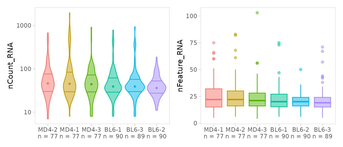
UMAP projections
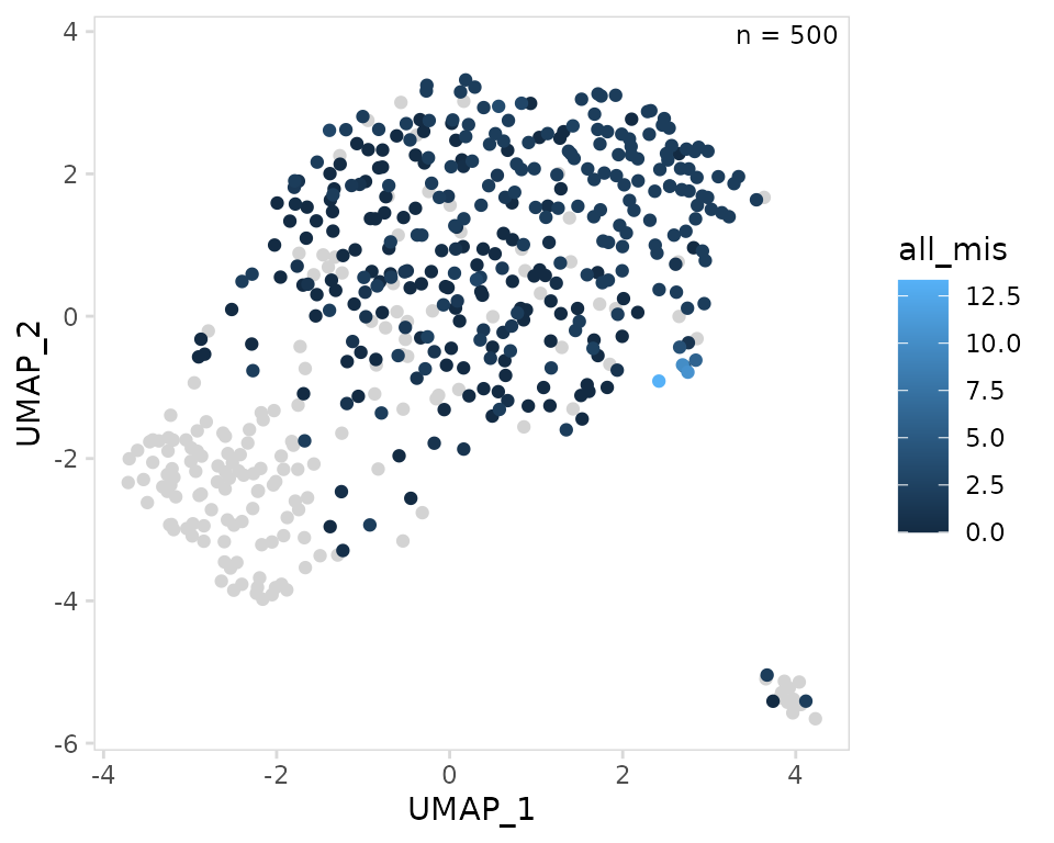
To plot V(D)J information on UMAP projections, the
plot_scatter() function can be used. By default this
function will plot the ‘UMAP_1’ and ‘UMAP_2’ columns on the x- and
y-axis. A function to use for summarizing per-chain values for each cell
must be specified using the summary_fn argument, by default
this is mean() for numeric data. Cells that lack V(D)J data
are stored as NAs in the object and will be shown on the
plot as light grey. The color used for plotting NAs can be
modified with the na_color argument.
In the example below, the mean number of mismatch mutations for each cell is shown.
so |>
  plot_scatter(
    data_col = "all_mis",
    na_color = "lightgrey"
  )
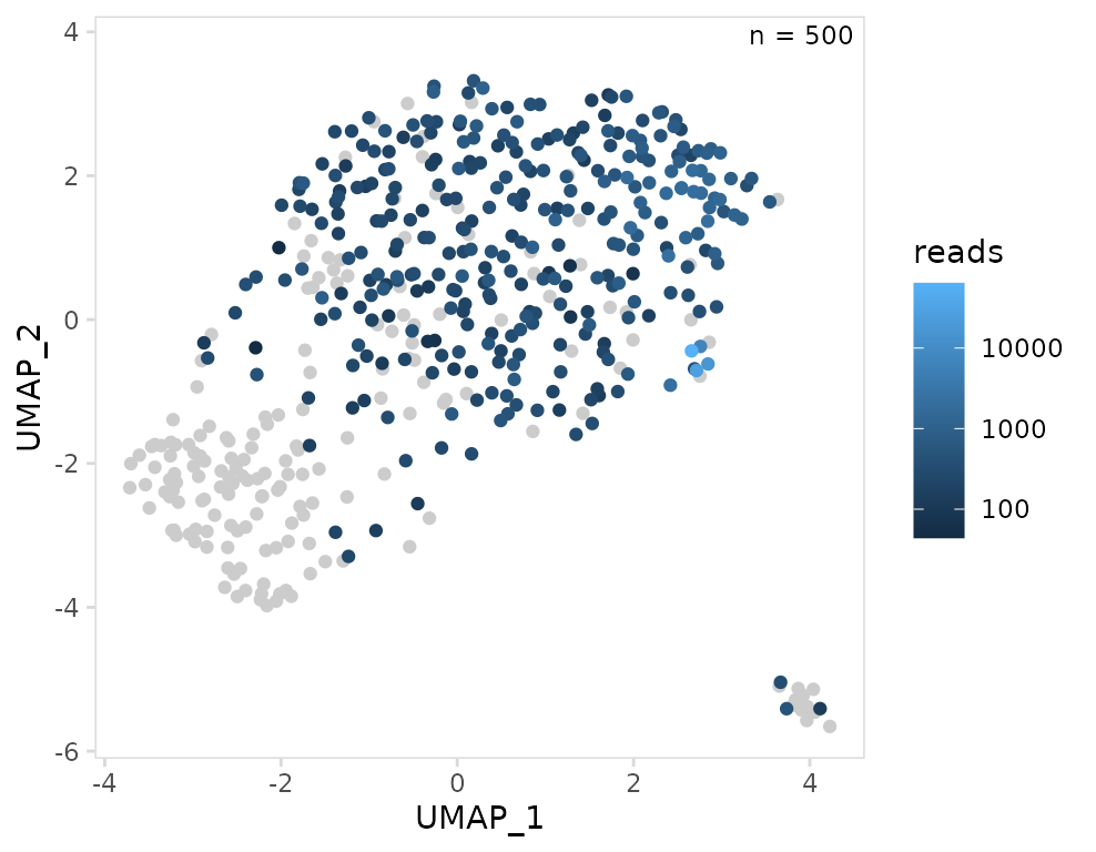
Instead of summarizing the per-chain values for each cell, we can
also specify a chain to use for plotting. In this example we are
plotting the CDR3 length for IGK chains. If a cell does not have an IGK
chain or has multiple IGK chains, it will be plotted as an
NA. Like other plotting functions, values can be
transformed using the trans argument.
so |>
  plot_scatter(
    data_col = "reads",
    chain    = "IGK",
    trans    = "log10"
  )
Cell clusters can be outlined by setting the outline
argument, this can help visualize points that are lightly colored.
u1 <- so |>
  plot_scatter(
    data_col    = "reads",
    plot_colors = c("white", "lightblue", "red"),
    trans       = "log10",
    size        = 2,
    outline     = TRUE
  )

u2 <- so |>
  plot_scatter(
    data_col    = "orig.ident",
    plot_colors = c("orange", "lightyellow"),
    size        = 2,
    outline     = TRUE
  )

u1 + u2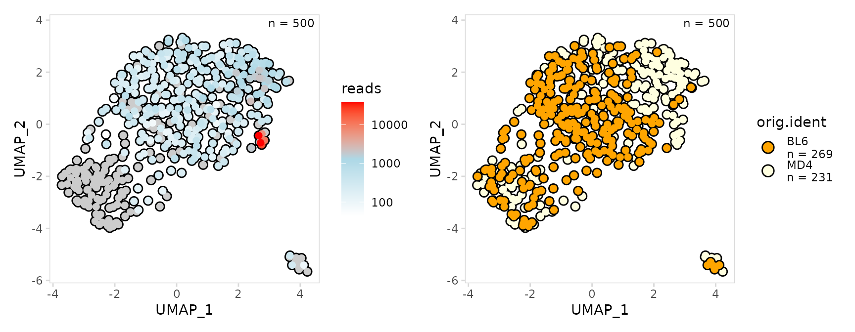
Plotting top clusters
To only plot the top clusters, the number of clusters to include can
be specified with the top argument. For
plot_violin(), clusters are ranked based on values in the
data_col column. For plot_scatter(), clusters
are ranked based on number of cells. Clusters can also be specified by
passing a vector of cluster names. The remaining cells are labeled using
the other_label argument.
# Show the top 3 clusters with highest values for nFeature_RNA
bx <- so |>
  plot_violin(
    data_col    = "nFeature_RNA",
    cluster_col = "seurat_clusters",
    method      = "boxplot",
    top         = 3
  )

# Select top clusters by passing a vector of names
u <- so |>
  plot_scatter(
    data_col = "seurat_clusters",
    top      = c("4", "1", "3")
  )

bx + u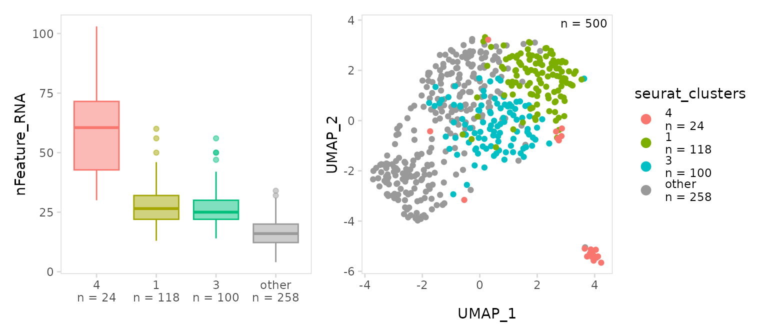
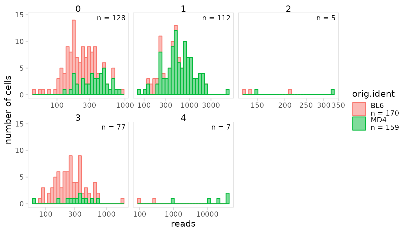
Splitting plots
Plots can be split into separate panels based on an additional
grouping variable using the group_col argument. The
arrangement of plot panels and the axis scales used for each panel can
be adjusted using the panel_nrow and
panel_scales arguments.
so |>
  plot_histogram(
    data_col    = "reads",
    cluster_col = "orig.ident",
    group_col   = "seurat_clusters",
    trans       = "log10",

    panel_nrow = 2,
    panel_scales = "free_x"
  )
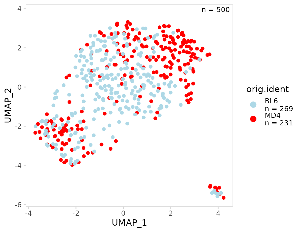
Plot aesthetics
Plot colors can be specified using the plot_colors
argument. This should be a vector of colors, to specify colors by
cluster name, a named vector can be passed. By default clusters are
ordered with the most abundant clusters on top. To modify this ordering,
a character vector can be passed to the plot_lvls
argument.
so |>
  plot_scatter(
    data_col    = "orig.ident",
    plot_colors = c(MD4 = "red", BL6 = "lightblue")
  )
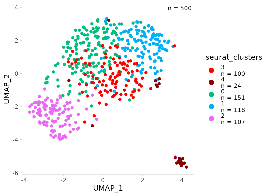
To only modify the color of a few clusters, a vector only containing
the clusters of interest can be passed. The same is true for the
plot_lvls argument, the name of a single cluster can be
passed to plot it on top.
In the example below we keep all the default colors except for clusters 3 and 4 and we specifically plot these clusters on top.
so |>
  plot_scatter(
    data_col    = "seurat_clusters",
    plot_colors = c("4" = "darkred", "3" = "red"),
    plot_lvls   = c("3", "4")
  )
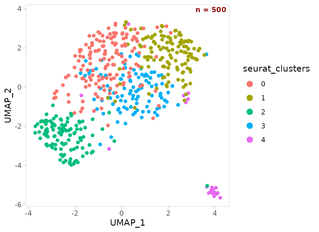
By default the number of data points plotted will be shown in the top
right corner, plot legend, and/or x-axis. The location of the label can
be specified using the n_label argument. Label appearance
can be modified by passing a named list of aesthetic parameters to the
label_params argument.
so |>
  plot_scatter(
    data_col     = "seurat_clusters",
    n_label      = "corner",
    label_params = list(color = "darkred", fontface = "bold")
  )
Session info
#> R version 4.3.1 (2023-06-16)
#> Platform: x86_64-pc-linux-gnu (64-bit)
#> Running under: Ubuntu 22.04.3 LTS
#>
#> Matrix products: default
#> BLAS:   /usr/lib/x86_64-linux-gnu/openblas-pthread/libblas.so.3
#> LAPACK: /usr/lib/x86_64-linux-gnu/openblas-pthread/libopenblasp-r0.3.20.so;  LAPACK version 3.10.0
#>
#> locale:
#>  [1] LC_CTYPE=C.UTF-8       LC_NUMERIC=C           LC_TIME=C.UTF-8
#>  [4] LC_COLLATE=C.UTF-8     LC_MONETARY=C.UTF-8    LC_MESSAGES=C.UTF-8
#>  [7] LC_PAPER=C.UTF-8       LC_NAME=C              LC_ADDRESS=C
#> [10] LC_TELEPHONE=C         LC_MEASUREMENT=C.UTF-8 LC_IDENTIFICATION=C
#>
#> time zone: UTC
#> tzcode source: system (glibc)
#>
#> attached base packages:
#> [1] stats     graphics  grDevices utils     datasets  methods   base
#>
#> other attached packages:
#> [1] ggplot2_3.4.4      SeuratObject_4.1.4 Seurat_4.4.0
#> [4] djvdj_0.1.0
#>
#> loaded via a namespace (and not attached):
#>   [1] RColorBrewer_1.1-3      jsonlite_1.8.7
#>   [3] magrittr_2.0.3          spatstat.utils_3.0-3
#>   [5] farver_2.1.1            rmarkdown_2.25
#>   [7] zlibbioc_1.46.0         fs_1.6.3
#>   [9] ragg_1.2.6              vctrs_0.6.4
#>  [11] ROCR_1.0-11             Rsamtools_2.16.0
#>  [13] memoise_2.0.1           spatstat.explore_3.2-5
#>  [15] RCurl_1.98-1.12         htmltools_0.5.6.1
#>  [17] sass_0.4.7              sctransform_0.4.1
#>  [19] parallelly_1.36.0       KernSmooth_2.23-21
#>  [21] bslib_0.5.1             htmlwidgets_1.6.2
#>  [23] desc_1.4.2              ica_1.0-3
#>  [25] plyr_1.8.9              plotly_4.10.3
#>  [27] zoo_1.8-12              cachem_1.0.8
#>  [29] igraph_1.5.1            mime_0.12
#>  [31] lifecycle_1.0.3         pkgconfig_2.0.3
#>  [33] Matrix_1.6-1.1          R6_2.5.1
#>  [35] fastmap_1.1.1           GenomeInfoDbData_1.2.10
#>  [37] fitdistrplus_1.1-11     future_1.33.0
#>  [39] shiny_1.7.5.1           digest_0.6.33
#>  [41] colorspace_2.1-0        S4Vectors_0.38.2
#>  [43] patchwork_1.1.3         rprojroot_2.0.3
#>  [45] tensor_1.5              irlba_2.3.5.1
#>  [47] GenomicRanges_1.52.1    textshaping_0.3.7
#>  [49] labeling_0.4.3          progressr_0.14.0
#>  [51] fansi_1.0.5             spatstat.sparse_3.0-2
#>  [53] httr_1.4.7              polyclip_1.10-6
#>  [55] abind_1.4-5             compiler_4.3.1
#>  [57] bit64_4.0.5             withr_2.5.1
#>  [59] BiocParallel_1.34.2     MASS_7.3-60
#>  [61] tools_4.3.1             lmtest_0.9-40
#>  [63] httpuv_1.6.12           future.apply_1.11.0
#>  [65] goftest_1.2-3           glue_1.6.2
#>  [67] nlme_3.1-162            promises_1.2.1
#>  [69] grid_4.3.1              Rtsne_0.16
#>  [71] cluster_2.1.4           reshape2_1.4.4
#>  [73] generics_0.1.3          gtable_0.3.4
#>  [75] spatstat.data_3.0-1     tzdb_0.4.0
#>  [77] tidyr_1.3.0             data.table_1.14.8
#>  [79] hms_1.1.3               XVector_0.40.0
#>  [81] sp_2.1-1                utf8_1.2.4
#>  [83] BiocGenerics_0.46.0     spatstat.geom_3.2-7
#>  [85] RcppAnnoy_0.0.21        ggrepel_0.9.4
#>  [87] RANN_2.6.1              pillar_1.9.0
#>  [89] stringr_1.5.0           vroom_1.6.4
#>  [91] later_1.3.1             splines_4.3.1
#>  [93] dplyr_1.1.3             lattice_0.21-8
#>  [95] bit_4.0.5               survival_3.5-5
#>  [97] deldir_1.0-9            ggtrace_0.2.0
#>  [99] tidyselect_1.2.0        Biostrings_2.68.1
#> [101] miniUI_0.1.1.1          pbapply_1.7-2
#> [103] knitr_1.44              gridExtra_2.3
#> [105] IRanges_2.34.1          scattermore_1.2
#> [107] stats4_4.3.1            xfun_0.40
#> [109] matrixStats_1.0.0       stringi_1.7.12
#> [111] lazyeval_0.2.2          yaml_2.3.7
#> [113] evaluate_0.22           codetools_0.2-19
#> [115] tibble_3.2.1            cli_3.6.1
#> [117] uwot_0.1.16             xtable_1.8-4
#> [119] reticulate_1.34.0       systemfonts_1.0.5
#> [121] munsell_0.5.0           jquerylib_0.1.4
#> [123] GenomeInfoDb_1.36.4     Rcpp_1.0.11
#> [125] globals_0.16.2          spatstat.random_3.2-1
#> [127] png_0.1-8               parallel_4.3.1
#> [129] ellipsis_0.3.2          pkgdown_2.0.7
#> [131] readr_2.1.4             bitops_1.0-7
#> [133] listenv_0.9.0           viridisLite_0.4.2
#> [135] scales_1.2.1            ggridges_0.5.4
#> [137] crayon_1.5.2            leiden_0.4.3
#> [139] purrr_1.0.2             rlang_1.1.1
#> [141] cowplot_1.1.1