Class 12: Working with gene lists

# run before class:
# devtools::install_github('rnabioco/practical-data-analysis')
# BiocManager::install("biomaRt")

library(pbda)
library(tidyverse)
library(cowplot)
library(gprofiler2)

Did experiment, ran through analysis pipeline, what now?

Handle gene lists

Try to connect prior knowledge to the results (genes you study, GO terms, or something like yeast_prot_prop)

Using some basic R and tibble manipulation commands

Retrieve gene lists from RNA-seq or scRNA-seq

Recall how data is saved in objects

Or whatever file you already saved containing lists of gene names

# from DESeq2 output, get a tibble back
# res <- results(dds)
# saveRDS(res, "res_class4.rds") # save any object from environment for next time
loc <- system.file("extdata", "res_class4.rds", package = 'pbda')
res <- readRDS(loc) # loading a DESeq2 object automatically loads DESeq2

head(res) # basically a dataframe
#> log2 fold change (MLE): drug none vs A 
#> Wald test p-value: drug none vs A 
#> DataFrame with 6 rows and 6 columns
#>                baseMean log2FoldChange     lfcSE      stat      pvalue
#>               <numeric>      <numeric> <numeric> <numeric>   <numeric>
#> WASH7P        10.003052      -0.121047  0.697033 -0.173661 8.62132e-01
#> MIR6859-1      1.707291      -0.496551  1.507128 -0.329468 7.41802e-01
#> LOC101927589   0.237587      -1.610617  4.370506 -0.368520 7.12486e-01
#> LOC729737    164.730908      -1.566207  0.264046 -5.931574 3.00045e-09
#> LOC100996442   0.456231      -1.575791  2.977488 -0.529235 5.96642e-01
#> LOC102723897 139.842022      -0.373916  0.214065 -1.746742 8.06821e-02
#>                     padj
#>                <numeric>
#> WASH7P       9.22818e-01
#> MIR6859-1    8.44449e-01
#> LOC101927589          NA
#> LOC729737    5.67484e-08
#> LOC100996442          NA
#> LOC102723897 1.81200e-01

res_tibble <- as_tibble(res, rownames = "gene")

res_tibble
#> # A tibble: 21,178 × 7
#>    gene          baseMean log2FoldChange lfcSE   stat      pvalue     padj
#>    <chr>            <dbl>          <dbl> <dbl>  <dbl>       <dbl>    <dbl>
#>  1 WASH7P          10.0           -0.121 0.697 -0.174     8.62e-1  9.23e-1
#>  2 MIR6859-1        1.71          -0.497 1.51  -0.329     7.42e-1  8.44e-1
#>  3 LOC101927589     0.238         -1.61  4.37  -0.369     7.12e-1 NA      
#>  4 LOC729737      165.            -1.57  0.264 -5.93      3.00e-9  5.67e-8
#>  5 LOC100996442     0.456         -1.58  2.98  -0.529     5.97e-1 NA      
#>  6 LOC102723897   140.            -0.374 0.214 -1.75      8.07e-2  1.81e-1
#>  7 LOC101929192     0.451         -1.58  3.00  -0.525     5.99e-1 NA      
#>  8 RP4-669L17.10    1.62          -1.13  1.41  -0.801     4.23e-1  5.94e-1
#>  9 LOC100134822     8.57           0.328 0.723  0.454     6.50e-1  7.80e-1
#> 10 MIR6723          0.616         -0.736 3.22  -0.229     8.19e-1 NA      
#> # … with 21,168 more rows

# res_tibble contains calculations for all genes, pick out "interesting" genes
gene_tibble <- res_tibble %>% 
  filter(!is.na(padj)) %>% # NA values from padj are from tossing low expressing genes
  filter(padj <= 0.01) %>% # padj <= 0.05 is common, or 0.01, sometimes even 0.1 is acceptable
  filter(log2FoldChange >= 1 | log2FoldChange <= -1) %>%
  arrange(desc(log2FoldChange))

gene_tibble
#> # A tibble: 1,908 × 7
#>    gene         baseMean log2FoldChange lfcSE  stat    pvalue      padj
#>    <chr>           <dbl>          <dbl> <dbl> <dbl>     <dbl>     <dbl>
#>  1 MAGEC2          133.           11.2  1.20   9.33 1.06e- 20 9.57e- 19
#>  2 PAGE5            76.5          10.7  1.20   8.90 5.57e- 19 4.23e- 17
#>  3 PGR            1732.            9.44 0.316 29.9  9.03e-197 7.88e-193
#>  4 FAM133A          27.2           9.24 1.24   7.44 1.01e- 13 4.05e- 12
#>  5 ZFP3             61.4           9.15 1.21   7.54 4.64e- 14 1.96e- 12
#>  6 GREB1          2343.            9.08 0.303 29.9  8.27e-197 7.88e-193
#>  7 LOC102724756     18.0           8.66 1.29   6.69 2.25e- 11 5.99e- 10
#>  8 CYP2B7P        1839.            8.58 0.336 25.5  1.94e-143 8.47e-140
#>  9 CTAG2           153.            8.31 0.675 12.3  7.76e- 35 2.46e- 32
#> 10 TMLHE           188.            8.25 1.05   7.88 3.34e- 15 1.62e- 13
#> # … with 1,898 more rows

# get top 10 down-regulated genes
gene_tibble_down10 <- gene_tibble %>%
  filter(log2FoldChange < 0) %>% 
  arrange(log2FoldChange) %>% 
  dplyr::slice(1:10) 

# get a vector of gene names
gene_vector <- gene_tibble$gene
gene_vector <- gene_tibble %>% pull(gene) # at least 5 more ways to do this

write_csv(gene_tibble, "gene_tibble.csv")

# or load already saved file on disk
loc <- system.file("extdata", "gene_tibble.csv", package = 'pbda')
gene_tibble2 <- read_csv(loc) # reads out as tibble

# or write as txt file, without col name
write_csv(gene_tibble %>% select(gene), "gene_tibble.txt", col_names = FALSE) # write from tibble
write_lines(gene_vector, "gene_tibble_v.txt") # write for vector

Gene set enrichment: feed gene lists to g:Profiler, get enrichment score back

g:Profiler https://biit.cs.ut.ee/gprofiler/

Here we consider the simple case of single, unordered lists of significantly differentially expressed human genes. g:Profiler can also handle ordered lists, other species, multiple lists in the same query, arbitry thresholds, several different multiple testing correction methods, arbitrary source selection, and much more.

# generate lists of singificantly up/downregulated genes from the RNA-seq example
upregulated_genes <- gene_tibble %>%
  filter(log2FoldChange >= 1, padj <= 0.01) %>%
  pull(gene)

downregulated_genes <- gene_tibble %>%
  filter(log2FoldChange <= -1, padj <= 0.01) %>%
  pull(gene)

# gost: gene list functional enrichment (for unordered human lists, only the list is required)
gost_up <- gost(upregulated_genes,
                organism = "hsapiens", 
                ordered_query = FALSE
                )

gost_down <- gost(downregulated_genes,
                organism = "hsapiens",
                ordered_query = FALSE)

# inspect the resulting gost output:
# meta slot contains information about the query, results and gene mapping
# All three print pretty unweildy lists, but can be very useful for troubleshooting
# gost_up$meta$query_metadata
# gost_up$meta$result_metadata
# gost_up$meta$genes_metadata 

# result slot contains the enrichment information
as_tibble(gost_up$result)
#> # A tibble: 235 × 14
#>    query   significant  p_value term_size query_size intersection_size
#>    <chr>   <lgl>          <dbl>     <int>      <int>             <int>
#>  1 query_1 TRUE        3.42e-14     11193        615               428
#>  2 query_1 TRUE        1.28e-13      4768        615               229
#>  3 query_1 TRUE        1.32e-12      2702        615               151
#>  4 query_1 TRUE        3.19e-12      6317        615               276
#>  5 query_1 TRUE        9.83e-12      5754        615               256
#>  6 query_1 TRUE        2.42e-11      4313        615               206
#>  7 query_1 TRUE        3.36e-10      3513        615               174
#>  8 query_1 TRUE        3.26e- 9     13001        615               460
#>  9 query_1 TRUE        5.11e- 9      7354        615               297
#> 10 query_1 TRUE        5.33e- 9      2425        615               130
#> # … with 225 more rows, and 8 more variables: precision <dbl>,
#> #   recall <dbl>, term_id <chr>, source <chr>, term_name <chr>,
#> #   effective_domain_size <int>, source_order <int>, parents <list>

# for a quick look a the results, we can plot the -log10 of top 20 entries in both lists
gost_log <- bind_rows(
  as_tibble(gost_up$result) %>%
    mutate(list = "up"),
  as_tibble(gost_down$result) %>%
    mutate(list = "down")
) %>%
  mutate(minus_log10 = -log10(p_value),
         list = factor(list, levels = c("up", "down"))) %>%
  group_by(list) %>%
  arrange(desc(minus_log10)) %>%
  dplyr::slice(1:20)

gost_log %>% select(list, term_name, minus_log10)
#> # A tibble: 40 × 3
#> # Groups:   list [2]
#>    list  term_name                           minus_log10
#>    <fct> <chr>                                     <dbl>
#>  1 up    regulation of cellular process            13.5 
#>  2 up    multicellular organism development        12.9 
#>  3 up    anatomical structure morphogenesis        11.9 
#>  4 up    developmental process                     11.5 
#>  5 up    anatomical structure development          11.0 
#>  6 up    system development                        10.6 
#>  7 up    animal organ development                   9.47
#>  8 up    biological regulation                      8.49
#>  9 up    multicellular organismal process           8.29
#> 10 up    regulation of developmental process        8.27
#> # … with 30 more rows

ggplot(gost_log, aes(x = reorder(term_name, minus_log10), y = minus_log10)) + #reorder Term by minus_log10
  geom_bar(stat = "identity") + # otherwise ggplot tries to count
  xlab("Term Name") +
  facet_wrap(~list, scales = "free") +
  coord_flip() +
  theme(axis.text.y = element_text(size = 7))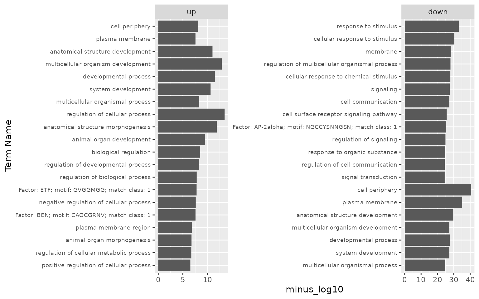


# adding source information for the enriched terms can also help with interpretation:
gost_log <- gost_log %>% mutate(term_name = paste(source,term_name, sep = ": ")) %>% select(list, term_name, minus_log10)

ggplot(gost_log, aes(x = reorder(term_name, minus_log10), y = minus_log10)) + #reorder Term by minus_log10
  geom_bar(stat = "identity") + # otherwise ggplot tries to count
  xlab("Term Name") +
  facet_wrap(~list, scales = "free") +
  coord_flip() +
  theme(axis.text.y = element_text(size = 7))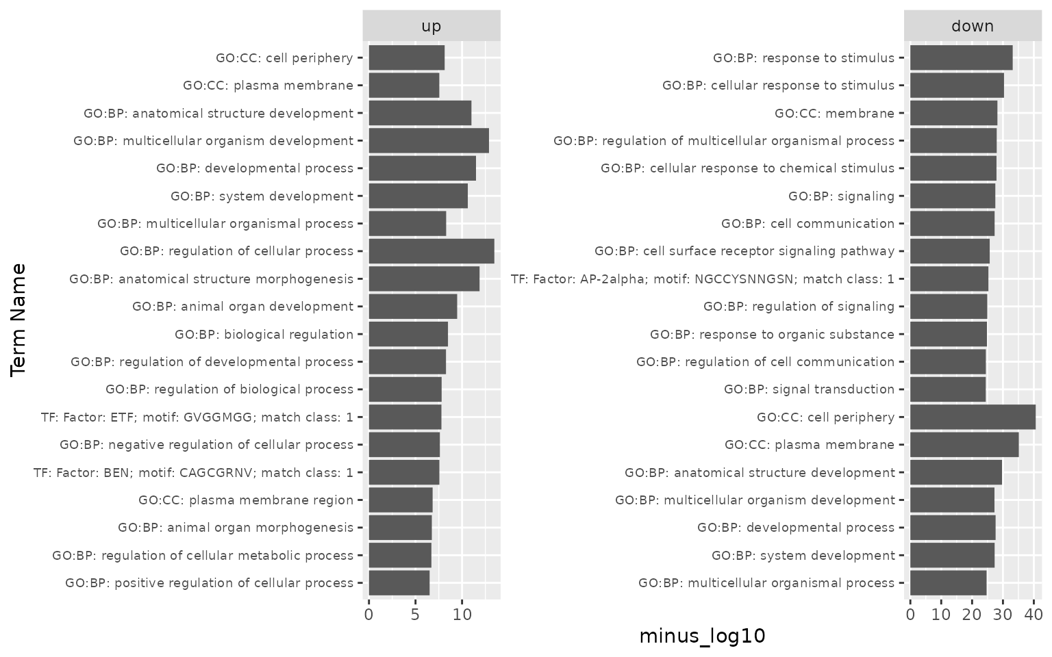

other options:

Panther http://www.geneontology.org/page/go-enrichment-analysis

GSEA (requires ranked list, for instance by fold-change, and requires full list of genes instead of just “significant”) http://software.broadinstitute.org/gsea/index.jsp

or, GO and GSEA right in R (will require additional packages):

topGO: https://bioconductor.org/packages/release/bioc/html/topGO.html

fgsea: http://bioconductor.org/packages/release/bioc/html/fgsea.html

Sometimes transformation of names is needed - `stringr` package, part of tidyverse

Depending on the transcriptome and analysis options used in RNA-seq/scRNA-seq, the list of names can be messy.

loc <- system.file("extdata", "ensg_tibble.csv", package = 'pbda')
ensg_tibble <- read_csv(loc)

ensg_tibble # those version numbers are often not recognized by software
#> # A tibble: 5 × 2
#>   gene                padj
#>   <chr>              <dbl>
#> 1 ENSG00000238164.4 0.0001
#> 2 ENSG00000049249.6 0.0002
#> 3 ENSG00000226823.1 0.0001
#> 4 ENSG00000266470.1 0.0002
#> 5 ENSG00000229435.2 0.05

str_replace: find and replace (run ?str_replace for documentation)

ensg_tibble_rm <- ensg_tibble %>% mutate(gene = str_replace(gene, 
                                                            pattern = "ENSG",
                                                            replacement = "#"))

ensg_tibble_rm
#> # A tibble: 5 × 2
#>   gene             padj
#>   <chr>           <dbl>
#> 1 #00000238164.4 0.0001
#> 2 #00000049249.6 0.0002
#> 3 #00000226823.1 0.0001
#> 4 #00000266470.1 0.0002
#> 5 #00000229435.2 0.05

# trimming of gene/transcript version
ensg_tibble2 <- ensg_tibble %>% mutate(gene_new = str_replace(gene, 
                                                          pattern = "\\..*", # . and everything after
                                                          replacement = "")) # empty string
# regular expressions are useful and worth the time to learn, see ?base::regex

ensg_tibble2
#> # A tibble: 5 × 3
#>   gene                padj gene_new       
#>   <chr>              <dbl> <chr>          
#> 1 ENSG00000238164.4 0.0001 ENSG00000238164
#> 2 ENSG00000049249.6 0.0002 ENSG00000049249
#> 3 ENSG00000226823.1 0.0001 ENSG00000226823
#> 4 ENSG00000266470.1 0.0002 ENSG00000266470
#> 5 ENSG00000229435.2 0.05   ENSG00000229435

# `separate` works too, if you want to keep the info
ensg_tibble3 <- ensg_tibble %>% separate(gene, into = c("gene", "version"), sep = "\\.")

# revisit the gprofiler output plot, clean up "term_name" column, stripping motif match info
gost_log2 <- gost_log %>% mutate(term_name = str_replace(term_name,
                                                         pattern = ";.*", # everything after and including ;
                                                         replacement = "")) %>%
  group_by(list, term_name) %>% # we now have duplicated term_names
  arrange(desc(minus_log10)) %>% # we arranges them by minus_log10
  dplyr::slice(1) # and take the most significant for each term

ggplot(gost_log2, aes(x = reorder(term_name, minus_log10), y = minus_log10)) + #reorder term_name by minus_log10
  geom_bar(stat = "identity") + # otherwise ggplot tries to count
  xlab("Term Name") +
  facet_wrap(~list, scales = "free") +
  coord_flip() +
  theme(axis.text.y = element_text(size = 7))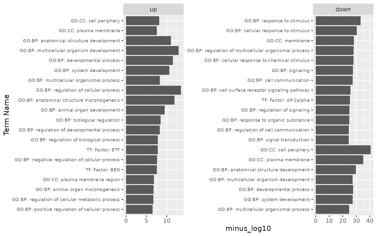

# to save plot
ggsave("gprofiler.png", plot = last_plot(), dpi = 300)

str_detect: spits out TRUE or FALSE

# "-AS" denotes antisense genes, we can find all those
str_detect(gene_tibble$gene, "-AS")[1:50]
#>  [1] FALSE FALSE FALSE FALSE FALSE FALSE FALSE FALSE FALSE FALSE FALSE
#> [12] FALSE FALSE FALSE FALSE FALSE FALSE FALSE FALSE FALSE FALSE FALSE
#> [23] FALSE FALSE FALSE FALSE  TRUE FALSE FALSE FALSE FALSE FALSE FALSE
#> [34] FALSE FALSE FALSE FALSE FALSE FALSE FALSE FALSE FALSE FALSE FALSE
#> [45] FALSE FALSE FALSE FALSE FALSE FALSE

# use in `filter`
gene_tibble_as <- gene_tibble %>% filter(str_detect(gene, "-AS"))

gene_tibble_as
#> # A tibble: 23 × 7
#>    gene       baseMean log2FoldChange lfcSE  stat   pvalue     padj
#>    <chr>         <dbl>          <dbl> <dbl> <dbl>    <dbl>    <dbl>
#>  1 ELOVL2-AS1     5.47           6.71 1.41   4.75 2.05e- 6 2.20e- 5
#>  2 GAS6-AS2      19.5            2.48 0.478  5.18 2.19e- 7 2.85e- 6
#>  3 ZEB1-AS1      26.3            2.22 0.423  5.26 1.45e- 7 1.96e- 6
#>  4 FGF13-AS1     12.1            1.99 0.576  3.46 5.44e- 4 3.06e- 3
#>  5 C1RL-AS1      30.9            1.49 0.416  3.58 3.46e- 4 2.07e- 3
#>  6 RAP2C-AS1     38.5            1.48 0.382  3.87 1.07e- 4 7.50e- 4
#>  7 KANSL1-AS1    30.8            1.45 0.455  3.19 1.42e- 3 6.91e- 3
#>  8 DPP10-AS1    115.             1.20 0.254  4.71 2.42e- 6 2.58e- 5
#>  9 CCNT2-AS1     43.7            1.18 0.319  3.70 2.14e- 4 1.37e- 3
#> 10 DHRS4-AS1    694.             1.13 0.170  6.65 2.98e-11 7.79e-10
#> # … with 13 more rows

str_c: concatenate strings

# also add annotations of our own
gene_tibble_as2 <- gene_tibble_as %>% mutate(gene = str_c("HUMAN-", gene))

gene_tibble_as2
#> # A tibble: 23 × 7
#>    gene             baseMean log2FoldChange lfcSE  stat   pvalue     padj
#>    <chr>               <dbl>          <dbl> <dbl> <dbl>    <dbl>    <dbl>
#>  1 HUMAN-ELOVL2-AS1     5.47           6.71 1.41   4.75 2.05e- 6 2.20e- 5
#>  2 HUMAN-GAS6-AS2      19.5            2.48 0.478  5.18 2.19e- 7 2.85e- 6
#>  3 HUMAN-ZEB1-AS1      26.3            2.22 0.423  5.26 1.45e- 7 1.96e- 6
#>  4 HUMAN-FGF13-AS1     12.1            1.99 0.576  3.46 5.44e- 4 3.06e- 3
#>  5 HUMAN-C1RL-AS1      30.9            1.49 0.416  3.58 3.46e- 4 2.07e- 3
#>  6 HUMAN-RAP2C-AS1     38.5            1.48 0.382  3.87 1.07e- 4 7.50e- 4
#>  7 HUMAN-KANSL1-AS1    30.8            1.45 0.455  3.19 1.42e- 3 6.91e- 3
#>  8 HUMAN-DPP10-AS1    115.             1.20 0.254  4.71 2.42e- 6 2.58e- 5
#>  9 HUMAN-CCNT2-AS1     43.7            1.18 0.319  3.70 2.14e- 4 1.37e- 3
#> 10 HUMAN-DHRS4-AS1    694.             1.13 0.170  6.65 2.98e-11 7.79e-10
#> # … with 13 more rows

str_sub: extract substrings

str_sub("HUMAN-ELOVL2-AS1", 2, 4)
#> [1] "UMA"

gene_tibble_as3 <- gene_tibble_as2 %>% mutate(gene = str_sub(gene, 2, 4))

gene_tibble_as3
#> # A tibble: 23 × 7
#>    gene  baseMean log2FoldChange lfcSE  stat   pvalue     padj
#>    <chr>    <dbl>          <dbl> <dbl> <dbl>    <dbl>    <dbl>
#>  1 UMA       5.47           6.71 1.41   4.75 2.05e- 6 2.20e- 5
#>  2 UMA      19.5            2.48 0.478  5.18 2.19e- 7 2.85e- 6
#>  3 UMA      26.3            2.22 0.423  5.26 1.45e- 7 1.96e- 6
#>  4 UMA      12.1            1.99 0.576  3.46 5.44e- 4 3.06e- 3
#>  5 UMA      30.9            1.49 0.416  3.58 3.46e- 4 2.07e- 3
#>  6 UMA      38.5            1.48 0.382  3.87 1.07e- 4 7.50e- 4
#>  7 UMA      30.8            1.45 0.455  3.19 1.42e- 3 6.91e- 3
#>  8 UMA     115.             1.20 0.254  4.71 2.42e- 6 2.58e- 5
#>  9 UMA      43.7            1.18 0.319  3.70 2.14e- 4 1.37e- 3
#> 10 UMA     694.             1.13 0.170  6.65 2.98e-11 7.79e-10
#> # … with 13 more rows

# to remove annotations of fixed length
gene_tibble_as4 <- gene_tibble_as2 %>% mutate(gene = str_sub(gene, 7, -5)) # extract just the gene name from "HUMAN-ELOVL2-AS1"

gene_tibble_as4
#> # A tibble: 23 × 7
#>    gene   baseMean log2FoldChange lfcSE  stat   pvalue     padj
#>    <chr>     <dbl>          <dbl> <dbl> <dbl>    <dbl>    <dbl>
#>  1 ELOVL2     5.47           6.71 1.41   4.75 2.05e- 6 2.20e- 5
#>  2 GAS6      19.5            2.48 0.478  5.18 2.19e- 7 2.85e- 6
#>  3 ZEB1      26.3            2.22 0.423  5.26 1.45e- 7 1.96e- 6
#>  4 FGF13     12.1            1.99 0.576  3.46 5.44e- 4 3.06e- 3
#>  5 C1RL      30.9            1.49 0.416  3.58 3.46e- 4 2.07e- 3
#>  6 RAP2C     38.5            1.48 0.382  3.87 1.07e- 4 7.50e- 4
#>  7 KANSL1    30.8            1.45 0.455  3.19 1.42e- 3 6.91e- 3
#>  8 DPP10    115.             1.20 0.254  4.71 2.42e- 6 2.58e- 5
#>  9 CCNT2     43.7            1.18 0.319  3.70 2.14e- 4 1.37e- 3
#> 10 DHRS4    694.             1.13 0.170  6.65 2.98e-11 7.79e-10
#> # … with 13 more rows

Various conversions in R - BioMart

BioMart can be used outside of R too: https://www.ensembl.org/biomart/martview

We will be using biomaRt

library(biomaRt)
# biomaRt contains many useful datasets
listDatasets(useMart("ENSEMBL_MART_ENSEMBL", host = "https://www.ensembl.org", )) %>% as_tibble() # hundreds of organisms

listAttributes(useMart("ensembl", dataset = "hsapiens_gene_ensembl")) %>% as_tibble() # thousands of rows/attributes

listFilters(useMart("ensembl", dataset = "hsapiens_gene_ensembl")) %>% as_tibble() # ways to filter the data

common usage 1: id to gene symbol conversion

human_mart <- useEnsembl("ensembl", dataset = "hsapiens_gene_ensembl", mirror = 'uswest') # assign the dataset to use

ensg_sym2 <- getBM(attributes = c("hgnc_symbol", "ensembl_gene_id"), # columns you want back
                 filters = "ensembl_gene_id",                       # type of info you are providing
                 mart = human_mart,                                 # dataset of certain species
                 values = ensg_tibble2$gene) %>% as_tibble()        # values of the filter

ensg_sym2

# try running this with ensg_tibble (version # intact), can't find matches

common usage 2: functional GO term annotation

listAttributes(useMart("ensembl", dataset = "hsapiens_gene_ensembl")) %>% 
  as_tibble() %>% 
  filter(str_detect(description, "GO")) # look at attributes related to GO

drerio_mart <- useEnsembl("ensembl", dataset = "drerio_gene_ensembl", mirror = 'uswest')

loc <- system.file("extdata", "genes_drerio.csv", package = 'pbda')
genes_drerio <- read_csv(loc)

genes_drerio

genesGO <- getBM(attributes = c("zfin_id_symbol", "go_id", "name_1006", "namespace_1003"), 
                 filters = "zfin_id_symbol", 
                 mart = drerio_mart, 
                 values = genes_drerio$gene, TRUE) %>% as_tibble()

genesGO

genesGO <- genesGO %>% filter(go_id != "") # note that there are lines with empty go terms, remember to remove those

# join GO dataframe with original RNA-seq/scRNA-seq data if needed
genes_drerio_joinedGO <- left_join(genes_drerio, genesGO, 
                                   by = c("gene" = "zfin_id_symbol"))

genes_drerio_joinedGO

# or, get all genes with GO term of interest, by providing multiple filters
genesGO_filtered <- getBM(attributes = c("zfin_id_symbol"), 
                  filters = c("zfin_id_symbol", "go"), 
                  mart = drerio_mart, 
                  values = list(genes_drerio$gene, c("GO:0003677")))

genesGO_filtered

common usage 3: ortholog conversion between species

# example of zebrafish to human gene symbol conversion
human_mart <- useEnsembl("ensembl", dataset = "hsapiens_gene_ensembl", mirror = 'uswest')
drerio_mart <- useEnsembl("ensembl", dataset = "drerio_gene_ensembl", mirror = 'uswest')

genes_human <- getLDS(attributes = c("hgnc_symbol"), # "linked datasets"
                      filters = "hgnc_symbol", 
                      mart = human_mart, 
                      attributesL = c("zfin_id_symbol"), 
                      martL = drerio_mart, 
                      values = genes_drerio$gene) %>% as_tibble()

genes_human

Exercise

Delete one argument from code above used to generate genesGO_filtered to obtain a list of all genes with GO id of “GO:0003677”.
Take a look at genesGO. Describe in pseudo-code, how you could add GO-CC back into the brauer_gene_exp.

Additional resources/reading

More sophisticated analysis than simply gene lists:

Find enriched sequence elements in promoters, UTRs, etc. See https://bedtools.readthedocs.io/en/latest/, http://meme-suite.org/, etc
WGCNA: weighted correlation network analysis
SCENIC: infer gene regulatory networks and cell types from single-cell RNA-seq data
Come to RBI office hours (Thursday 1-2:30)!

Rui Fu & Austin Gillen

2022-07-06

Did experiment, ran through analysis pipeline, what now?

Retrieve gene lists from RNA-seq or scRNA-seq

Gene set enrichment: feed gene lists to g:Profiler, get enrichment score back

Sometimes transformation of names is needed - `stringr` package, part of tidyverse

Various conversions in R - BioMart

Exercise

Additional resources/reading

Class 12: Working with gene lists

Rui Fu & Austin Gillen

2022-07-06

Did experiment, ran through analysis pipeline, what now?

Retrieve gene lists from RNA-seq or scRNA-seq

Gene set enrichment: feed gene lists to g:Profiler, get enrichment score back

Sometimes transformation of names is needed - stringr package, part of tidyverse

Various conversions in R - BioMart

Exercise

Additional resources/reading

Sometimes transformation of names is needed - `stringr` package, part of tidyverse