Class 1: Course Overview | Data Import and Tidying • pbda

Goals for the course

Master the basics of data import, processing, plotting, and report generation in RStudio.
Get hooked on RStudio instead of MS Excel, Prism, etc as your go-to analysis software.
Learn productive analysis habits.
Understand the analysis ecosystem so that new types of data are easily approachable

RStudio Overview

The class has its own R package, so you should begin by loading it into your session. You will need to reinstall the package when we make updates.

# devtools::install_github('rnabioco/practical-data-analysis')
library(pbda)

Environment

The Environment panel enables data import and environment browsing.

There are two main ways to import data within RStudio. One is interactive, using the “Import Dataset” button in the Environment panel.

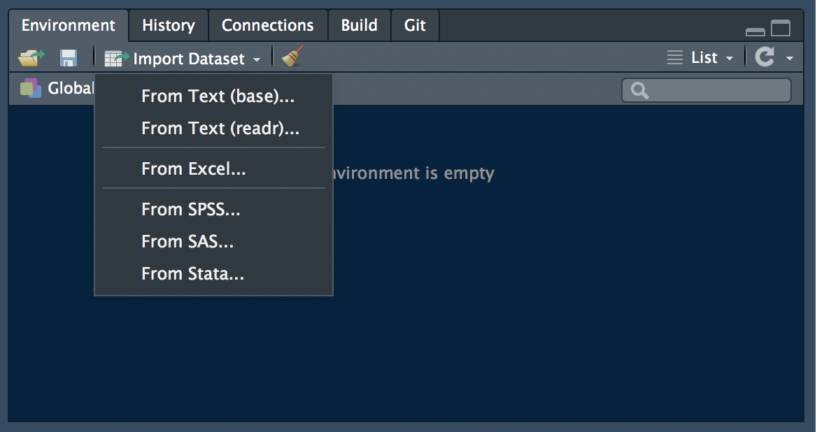
data import

`read` functions

Alternatively you can use functions in readr and readxl to load data on the console or within an RMarkdown report. All of the functions have read_* prefixes.

library(readr)
read_csv(readr_example("mtcars.csv"))
#> Rows: 32 Columns: 11
#> ── Column specification ──────────────────────────────────────────────────
#> Delimiter: ","
#> dbl (11): mpg, cyl, disp, hp, drat, wt, qsec, vs, am, gear, carb
#> 
#> ℹ Use `spec()` to retrieve the full column specification for this data.
#> ℹ Specify the column types or set `show_col_types = FALSE` to quiet this message.
#> # A tibble: 32 × 11
#>      mpg   cyl  disp    hp  drat    wt  qsec    vs    am  gear  carb
#>    <dbl> <dbl> <dbl> <dbl> <dbl> <dbl> <dbl> <dbl> <dbl> <dbl> <dbl>
#>  1  21       6  160    110  3.9   2.62  16.5     0     1     4     4
#>  2  21       6  160    110  3.9   2.88  17.0     0     1     4     4
#>  3  22.8     4  108     93  3.85  2.32  18.6     1     1     4     1
#>  4  21.4     6  258    110  3.08  3.22  19.4     1     0     3     1
#>  5  18.7     8  360    175  3.15  3.44  17.0     0     0     3     2
#>  6  18.1     6  225    105  2.76  3.46  20.2     1     0     3     1
#>  7  14.3     8  360    245  3.21  3.57  15.8     0     0     3     4
#>  8  24.4     4  147.    62  3.69  3.19  20       1     0     4     2
#>  9  22.8     4  141.    95  3.92  3.15  22.9     1     0     4     2
#> 10  19.2     6  168.   123  3.92  3.44  18.3     1     0     4     4
#> # … with 22 more rows

library(readxl)
read_excel(readxl_example("datasets.xlsx"))
#> # A tibble: 150 × 5
#>    Sepal.Length Sepal.Width Petal.Length Petal.Width Species
#>           <dbl>       <dbl>        <dbl>       <dbl> <chr>  
#>  1          5.1         3.5          1.4         0.2 setosa 
#>  2          4.9         3            1.4         0.2 setosa 
#>  3          4.7         3.2          1.3         0.2 setosa 
#>  4          4.6         3.1          1.5         0.2 setosa 
#>  5          5           3.6          1.4         0.2 setosa 
#>  6          5.4         3.9          1.7         0.4 setosa 
#>  7          4.6         3.4          1.4         0.3 setosa 
#>  8          5           3.4          1.5         0.2 setosa 
#>  9          4.4         2.9          1.4         0.2 setosa 
#> 10          4.9         3.1          1.5         0.1 setosa 
#> # … with 140 more rows

You can also explore your environment with the “Global Environment” button.

Console

The Console panel enables interactive analysis.

library(tidyverse)
#> ── Attaching packages ───────────────────────────────── tidyverse 1.3.1 ──
#> ✔ ggplot2 3.3.6     ✔ dplyr   1.0.9
#> ✔ tibble  3.1.7     ✔ stringr 1.4.0
#> ✔ tidyr   1.2.0     ✔ forcats 0.5.1
#> ✔ purrr   0.3.4
#> ── Conflicts ──────────────────────────────────── tidyverse_conflicts() ──
#> ✖ dplyr::filter() masks stats::filter()
#> ✖ dplyr::lag()    masks stats::lag()

This one invocation loads several libraries including dplyr and ggplot2.

Viewer

The tidyverse contains ggplot2, which you covered in your pre-requisites. Let’s make a simple plot in RStudio. Note that the plot appears in the “Plots” panel. From there, you can Zoom, Export to a file, or Publish on RPubs.

library(ggplot2)
ggplot(mtcars, aes(x = hp, y = mpg, color = factor(cyl))) + geom_point()

Editor

Finally we’ll create an RMarkdown document in the Editor panel. Select File > New File > RMarkdown… and fill the Title and Author fields. Then click OK to create an RMarkdown document. When you have completed editing the document, click the “Knit” button to render the output (e.g., as an HTML page).

Rmarkdown is customizable with tables of contents, tabbed views and more. See the Rmarkdown documentation for examples.

Projects

RStudio provides a “Project” concept to keep related analyses together. I suggest starting each class by making your own project (File > New Project).

Tidyverse cheatsheets

See Help > Cheatsheets for helpful references. Print them out and pin them up next to your screen. The dplyr and ggplot2 cheatsheets are especially useful for beginners.

Git and Github

Github provides several advantages:

Revision control. You have a history of all changes to your documents and can go back to any point.
Collaboration. It is easy to share analyses with your colleagues and is built to enable multiple people to work an a common project.
Publicity. Your github page reflects your interests and productivity. Others might visit to evaluate your code samples.

Jenny Bryan’s “Happy Git with R” tutorial gets you up and running by integrating Git and R Studio.

We’ll be using github to submit problem sets, so make sure this is set up by class time on Thursday.

Formatting data for efficient analysis

Reformatting your data into “tidy” format is a useful practice that allows you efficiently manipulate and analyze data. We will start with some toy examples and then will reformat a commonly used data type from a quantitative PCR experiment.

Tidy data adopts three simple conventions:

Columns are variables.
Rows are observations.
Store related data in separate tables.

The `tibble`

A tibble is similar to a data.frame with some important differences. A tibble provides a quick overview of your data including its structure (rows and columns) and column types. Use as_tibble() to convert a data.frame:

head(iris)
#>   Sepal.Length Sepal.Width Petal.Length Petal.Width Species
#> 1          5.1         3.5          1.4         0.2  setosa
#> 2          4.9         3.0          1.4         0.2  setosa
#> 3          4.7         3.2          1.3         0.2  setosa
#> 4          4.6         3.1          1.5         0.2  setosa
#> 5          5.0         3.6          1.4         0.2  setosa
#> 6          5.4         3.9          1.7         0.4  setosa

library(tidyverse)
as_tibble(iris)
#> # A tibble: 150 × 5
#>    Sepal.Length Sepal.Width Petal.Length Petal.Width Species
#>           <dbl>       <dbl>        <dbl>       <dbl> <fct>  
#>  1          5.1         3.5          1.4         0.2 setosa 
#>  2          4.9         3            1.4         0.2 setosa 
#>  3          4.7         3.2          1.3         0.2 setosa 
#>  4          4.6         3.1          1.5         0.2 setosa 
#>  5          5           3.6          1.4         0.2 setosa 
#>  6          5.4         3.9          1.7         0.4 setosa 
#>  7          4.6         3.4          1.4         0.3 setosa 
#>  8          5           3.4          1.5         0.2 setosa 
#>  9          4.4         2.9          1.4         0.2 setosa 
#> 10          4.9         3.1          1.5         0.1 setosa 
#> # … with 140 more rows

The `tidyr` package

The tidyr package has useful functions to format data for efficient analysis. See the cheat sheet for reference.

`gather` and `spread`

These are the workhorse functions in tidyr. Use gather when variables are in columns and you want them in tidy format.

library(pbda)
# column names in "wide" format are variables
mtcars_tbl
#> # A tibble: 32 × 12
#>    name    mpg   cyl  disp    hp  drat    wt  qsec    vs    am  gear  carb
#>    <chr> <dbl> <dbl> <dbl> <dbl> <dbl> <dbl> <dbl> <dbl> <dbl> <dbl> <dbl>
#>  1 Mazd…  21       6  160    110  3.9   2.62  16.5     0     1     4     4
#>  2 Mazd…  21       6  160    110  3.9   2.88  17.0     0     1     4     4
#>  3 Dats…  22.8     4  108     93  3.85  2.32  18.6     1     1     4     1
#>  4 Horn…  21.4     6  258    110  3.08  3.22  19.4     1     0     3     1
#>  5 Horn…  18.7     8  360    175  3.15  3.44  17.0     0     0     3     2
#>  6 Vali…  18.1     6  225    105  2.76  3.46  20.2     1     0     3     1
#>  7 Dust…  14.3     8  360    245  3.21  3.57  15.8     0     0     3     4
#>  8 Merc…  24.4     4  147.    62  3.69  3.19  20       1     0     4     2
#>  9 Merc…  22.8     4  141.    95  3.92  3.15  22.9     1     0     4     2
#> 10 Merc…  19.2     6  168.   123  3.92  3.44  18.3     1     0     4     4
#> # … with 22 more rows

# gather variables and observations into `key` and `value` columns - so-called "long" format
xx <- mtcars_tbl %>% gather(key, value, -name)
xx
#> # A tibble: 352 × 3
#>    name              key   value
#>    <chr>             <chr> <dbl>
#>  1 Mazda RX4         mpg    21  
#>  2 Mazda RX4 Wag     mpg    21  
#>  3 Datsun 710        mpg    22.8
#>  4 Hornet 4 Drive    mpg    21.4
#>  5 Hornet Sportabout mpg    18.7
#>  6 Valiant           mpg    18.1
#>  7 Duster 360        mpg    14.3
#>  8 Merc 240D         mpg    24.4
#>  9 Merc 230          mpg    22.8
#> 10 Merc 280          mpg    19.2
#> # … with 342 more rows

# and convert back to "wide" format
xx %>% spread(key, value)
#> # A tibble: 32 × 12
#>    name     am  carb   cyl  disp  drat  gear    hp   mpg  qsec    vs    wt
#>    <chr> <dbl> <dbl> <dbl> <dbl> <dbl> <dbl> <dbl> <dbl> <dbl> <dbl> <dbl>
#>  1 AMC …     0     2     8 304    3.15     3   150  15.2  17.3     0  3.44
#>  2 Cadi…     0     4     8 472    2.93     3   205  10.4  18.0     0  5.25
#>  3 Cama…     0     4     8 350    3.73     3   245  13.3  15.4     0  3.84
#>  4 Chry…     0     4     8 440    3.23     3   230  14.7  17.4     0  5.34
#>  5 Dats…     1     1     4 108    3.85     4    93  22.8  18.6     1  2.32
#>  6 Dodg…     0     2     8 318    2.76     3   150  15.5  16.9     0  3.52
#>  7 Dust…     0     4     8 360    3.21     3   245  14.3  15.8     0  3.57
#>  8 Ferr…     1     6     6 145    3.62     5   175  19.7  15.5     0  2.77
#>  9 Fiat…     1     1     4  78.7  4.08     4    66  32.4  19.5     1  2.2 
#> 10 Fiat…     1     1     4  79    4.08     4    66  27.3  18.9     1  1.94
#> # … with 22 more rows

Long format

Each form has its advantages. For example, long format makes it easy to calculate summaries:

xx %>% group_by(key) %>% summarize(median(value))
#> # A tibble: 11 × 2
#>    key   `median(value)`
#>    <chr>           <dbl>
#>  1 am               0   
#>  2 carb             2   
#>  3 cyl              6   
#>  4 disp           196.  
#>  5 drat             3.70
#>  6 gear             4   
#>  7 hp             123   
#>  8 mpg             19.2 
#>  9 qsec            17.7 
#> 10 vs               0   
#> 11 wt               3.32

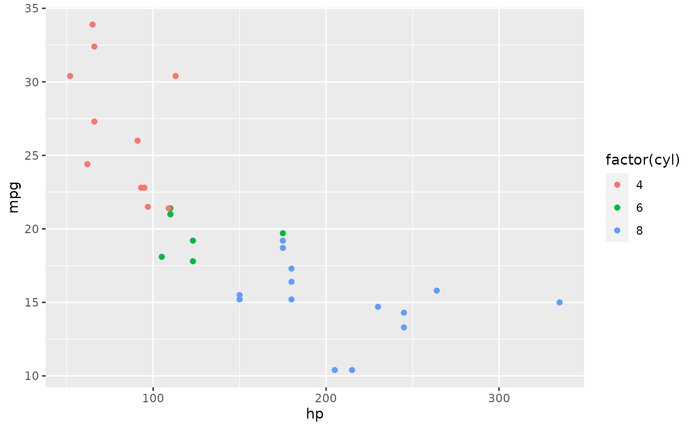
Wide format

And wide format is useful for plotting.

library(ggrepel)

set.seed(42)
ggplot(mtcars_tbl) +
  geom_point(aes(hp, mpg, size = 5)) +
  geom_label_repel(aes(hp, mpg, fill = factor(cyl), label = name))
#> Warning: ggrepel: 5 unlabeled data points (too many overlaps). Consider
#> increasing max.overlaps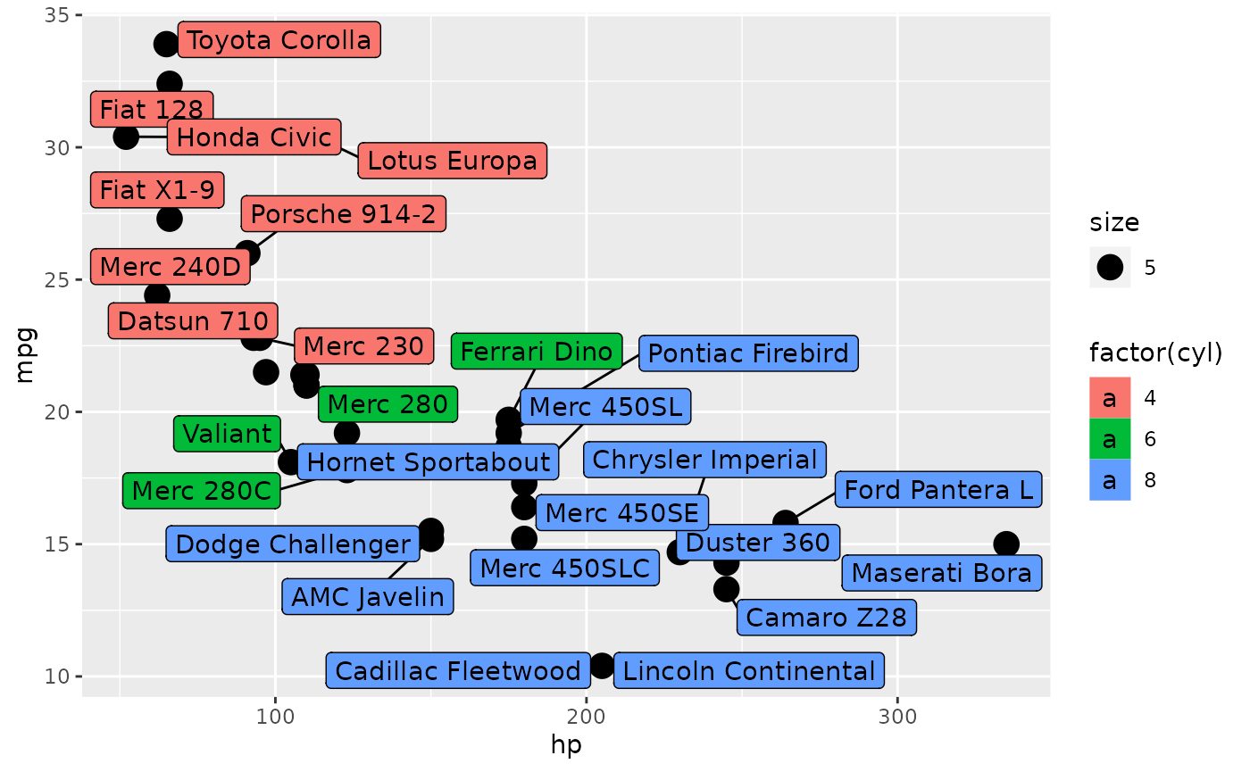

Exercise

Examine the beavers data set (beaver1 and beaver2) to identify its variables. Is it in tidy format? If not, how would you rearrange it to make it tidy?

`separate` and `unite`

separate takes a column containing multiple variables on input and returns multiple columns, each with a new variable. For example, a column with year/month/day information can be separated into invidual columns.

ys <- 1999:2002
ms <- c('Jan', 'Feb', 'Mar')
ds <- 1:10

dates <- tidyr::crossing(ys, ms, ds) %>% unite(date, ys:ds, sep = '-')

`separate`

dates
#> # A tibble: 120 × 1
#>    date       
#>    <chr>      
#>  1 1999-Feb-1 
#>  2 1999-Feb-2 
#>  3 1999-Feb-3 
#>  4 1999-Feb-4 
#>  5 1999-Feb-5 
#>  6 1999-Feb-6 
#>  7 1999-Feb-7 
#>  8 1999-Feb-8 
#>  9 1999-Feb-9 
#> 10 1999-Feb-10
#> # … with 110 more rows

# separate is the inverse of unite
dates %>% separate(date, into = c('year', 'month', 'day'), sep = '-')
#> # A tibble: 120 × 3
#>    year  month day  
#>    <chr> <chr> <chr>
#>  1 1999  Feb   1    
#>  2 1999  Feb   2    
#>  3 1999  Feb   3    
#>  4 1999  Feb   4    
#>  5 1999  Feb   5    
#>  6 1999  Feb   6    
#>  7 1999  Feb   7    
#>  8 1999  Feb   8    
#>  9 1999  Feb   9    
#> 10 1999  Feb   10   
#> # … with 110 more rows

The sep argument can take:

a character (split rep_value using sep = '_' into rep and value)
a position (split a1 using sep = 1 into a and 1)

Finally the extra and fill arguments to separate control what happens when there are too many and not enough variables.

`crossing` and `complete`

crossing is useful for generating combinations of variables in tibble format. For example, use crossing to generate combinations of experimental varaibles including sample names, gene names, reaction conditions, and replicates.

genotype <- c('wt', 'mut')
gene <- c('IFN', 'ACTIN')
time <- c(0, 12, 24, 48)
rt <- c('+', '-') # reverse transcriptase added?
rep <- 1:3

samples <- tidyr::crossing(genotype, gene, time, rep, rt)

samples
#> # A tibble: 96 × 5
#>    genotype gene   time   rep rt   
#>    <chr>    <chr> <dbl> <int> <chr>
#>  1 mut      ACTIN     0     1 -    
#>  2 mut      ACTIN     0     1 +    
#>  3 mut      ACTIN     0     2 -    
#>  4 mut      ACTIN     0     2 +    
#>  5 mut      ACTIN     0     3 -    
#>  6 mut      ACTIN     0     3 +    
#>  7 mut      ACTIN    12     1 -    
#>  8 mut      ACTIN    12     1 +    
#>  9 mut      ACTIN    12     2 -    
#> 10 mut      ACTIN    12     2 +    
#> # … with 86 more rows

Data in the 96-well plate format.

Now we’ll use tidy data principles to analyze some qPCR data.

Many biological assays make use of the 96 (or 384) well plate. Note the similarity between the plate and a tibble: there are rows and columns, and each well contains a reaction that will generate one or more data points.

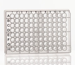
plate

Sample names

All variables should be systematically listed in your sample names, i.e. name_rep_time_RT. Systematic naming makes it easy to extract relevant information.

Take this example, where the sample names are a combination of a genotype (WT and MT), a time point (0,4,8,24 hour), and a replicate (1,2,3), separated by a hyphen.

#> # A tibble: 24 × 2
#>    sample.name value
#>    <chr>       <int>
#>  1 MT-t0-1        71
#>  2 MT-t0-2        77
#>  3 MT-t0-3        51
#>  4 MT-t24-1       88
#>  5 MT-t24-2       50
#>  6 MT-t24-3       90
#>  7 MT-t4-1        67
#>  8 MT-t4-2         9
#>  9 MT-t4-3        84
#> 10 MT-t8-1        29
#> # … with 14 more rows

Extracting sample names

Because the samples have systematic names, it is easy to separate this information into individual columns.

sample_info <- samples %>%
  tidyr::separate(
    sample.name,
    into = c('sample', 'hour', 'rep'),
    sep = "-"
  )

sample_info
#> # A tibble: 24 × 4
#>    sample hour  rep   value
#>    <chr>  <chr> <chr> <int>
#>  1 MT     t0    1        71
#>  2 MT     t0    2        77
#>  3 MT     t0    3        51
#>  4 MT     t24   1        88
#>  5 MT     t24   2        50
#>  6 MT     t24   3        90
#>  7 MT     t4    1        67
#>  8 MT     t4    2         9
#>  9 MT     t4    3        84
#> 10 MT     t8    1        29
#> # … with 14 more rows

Data manipulation

Now we can use dplyr and tidyr functions to manipulate the data.

# calculate summary statistics
sample_info %>% group_by(sample, hour) %>% summarize(mean(value))
#> `summarise()` has grouped output by 'sample'. You can override using the
#> `.groups` argument.
#> # A tibble: 8 × 3
#> # Groups:   sample [2]
#>   sample hour  `mean(value)`
#>   <chr>  <chr>         <dbl>
#> 1 MT     t0             66.3
#> 2 MT     t24            76  
#> 3 MT     t4             53.3
#> 4 MT     t8             57.3
#> 5 WT     t0             28  
#> 6 WT     t24            69.7
#> 7 WT     t4             51  
#> 8 WT     t8             35.7

# subtract a background value. N.B.: rearranging the table makes this calculation easy.
sample_info %>% spread(hour, value) %>% mutate(t24_norm = t24 - t0)
#> # A tibble: 6 × 7
#>   sample rep      t0   t24    t4    t8 t24_norm
#>   <chr>  <chr> <int> <int> <int> <int>    <int>
#> 1 MT     1        71    88    67    29       17
#> 2 MT     2        77    50     9    78      -27
#> 3 MT     3        51    90    84    65       39
#> 4 WT     1        53    66    60    22       13
#> 5 WT     2         7    82    57    32       75
#> 6 WT     3        24    61    36    53       37

qPCR data

The class library provides two related tibbles that describe a simulated qPCR experiment called qpcr_names and qpcr_data.

library(pbda)

qpcr_names
#> # A tibble: 8 × 13
#>   row   `1`    `2`   `3`   `4`   `5`   `6`   `7`   `8`   `9`   `10`  `11` 
#>   <chr> <chr>  <chr> <chr> <chr> <chr> <chr> <chr> <chr> <chr> <chr> <chr>
#> 1 A     mut_0… mut_… mut_… mut_… mut_… mut_… wt_0… wt_0… wt_1… wt_2… wt_2…
#> 2 B     mut_0… mut_… mut_… mut_… mut_… mut_… wt_0… wt_0… wt_1… wt_2… wt_2…
#> 3 C     mut_0… mut_… mut_… mut_… mut_… mut_… wt_0… wt_0… wt_1… wt_2… wt_2…
#> 4 D     mut_0… mut_… mut_… mut_… mut_… mut_… wt_0… wt_0… wt_1… wt_2… wt_2…
#> 5 E     mut_0… mut_… mut_… mut_… mut_… mut_… wt_0… wt_1… wt_1… wt_2… wt_4…
#> 6 F     mut_0… mut_… mut_… mut_… mut_… mut_… wt_0… wt_1… wt_1… wt_2… wt_4…
#> 7 G     mut_0… mut_… mut_… mut_… mut_… mut_… wt_0… wt_1… wt_1… wt_2… wt_4…
#> 8 H     mut_0… mut_… mut_… mut_… mut_… mut_… wt_0… wt_1… wt_1… wt_2… wt_4…
#> # … with 1 more variable: `12` <chr>

qpcr_data
#> # A tibble: 8 × 13
#>   row     `1`   `2`   `3`   `4`   `5`   `6`   `7`   `8`   `9`  `10`  `11`
#>   <chr> <dbl> <dbl> <dbl> <dbl> <dbl> <dbl> <dbl> <dbl> <dbl> <dbl> <dbl>
#> 1 A       2.6  10.5   9.2  20    146.  83.6   2.4  10.5  10.4  19    146.
#> 2 B       0     0     0     0      0    0     0     0     0     0      0 
#> 3 C       1.6  16.5  79.5  20    146. 680.    1.2  12    78    19.2  144 
#> 4 D       0     0     0     0      0    0     0     0     0     0      0 
#> 5 E       2.8  11    79.5  19.8  105  663     2     9    69    19.8   71 
#> 6 F       0     0     0     0      0    0     0     0     0     0      0 
#> 7 G      12     9.8  78   144    116  774    22.5  11    73.5 146.   118.
#> 8 H       0     0     0     0      0    0     0     0     0     0      0 
#> # … with 1 more variable: `12` <dbl>

We will use tidying concepts to prepare this data for efficient analysis and visualization.

qPCR data tidying

Tidy qpcr_data and qpcr_names into a structure like:

#> # A tibble: 96 × 3
#>    row   col     exp
#>    <chr> <chr> <dbl>
#>  1 A     1       2.6
#>  2 B     1       0  
#>  3 C     1       1.6
#>  4 D     1       0  
#>  5 E     1       2.8
#>  6 F     1       0  
#>  7 G     1      12  
#>  8 H     1       0  
#>  9 A     2      10.5
#> 10 B     2       0  
#> # … with 86 more rows

Sample names

Separate variables into new columns in qpcr_names_tidy.

#> # A tibble: 96 × 7
#>    row   col   sample time  gene  rt    rep  
#>    <chr> <chr> <chr>  <chr> <chr> <chr> <chr>
#>  1 A     1     mut    0     ACTIN +     1    
#>  2 B     1     mut    0     ACTIN -     1    
#>  3 C     1     mut    0     ACTIN +     2    
#>  4 D     1     mut    0     ACTIN -     2    
#>  5 E     1     mut    0     ACTIN +     3    
#>  6 F     1     mut    0     ACTIN -     3    
#>  7 G     1     mut    0     IFN   +     1    
#>  8 H     1     mut    0     IFN   -     1    
#>  9 A     2     mut    0     IFN   +     2    
#> 10 B     2     mut    0     IFN   -     2    
#> # … with 86 more rows

Data joining

Join the tidied data together.

#> Joining, by = c("row", "col")
#> # A tibble: 96 × 8
#>    row   col   sample time  gene  rt    rep     exp
#>    <chr> <chr> <chr>  <chr> <chr> <chr> <chr> <dbl>
#>  1 A     1     mut    0     ACTIN +     1       2.6
#>  2 B     1     mut    0     ACTIN -     1       0  
#>  3 C     1     mut    0     ACTIN +     2       1.6
#>  4 D     1     mut    0     ACTIN -     2       0  
#>  5 E     1     mut    0     ACTIN +     3       2.8
#>  6 F     1     mut    0     ACTIN -     3       0  
#>  7 G     1     mut    0     IFN   +     1      12  
#>  8 H     1     mut    0     IFN   -     1       0  
#>  9 A     2     mut    0     IFN   +     2      10.5
#> 10 B     2     mut    0     IFN   -     2       0  
#> # … with 86 more rows

Statistical summary

Calculate summary statistics for each gene, cell and time point across replicates.

qpcr_tidy %>%
  filter(rt == "+") %>%
  group_by(sample, gene, time) %>%
  summarize(mean_exp = mean(exp), var_exp = var(exp))
#> `summarise()` has grouped output by 'sample', 'gene'. You can override
#> using the `.groups` argument.
#> # A tibble: 16 × 5
#> # Groups:   sample, gene [4]
#>    sample gene  time  mean_exp   var_exp
#>    <chr>  <chr> <chr>    <dbl>     <dbl>
#>  1 mut    ACTIN 0         2.33    0.413 
#>  2 mut    ACTIN 12       10       0.840 
#>  3 mut    ACTIN 24       19.9     0.0133
#>  4 mut    ACTIN 48      102.    271.    
#>  5 mut    IFN   0        13       9.75  
#>  6 mut    IFN   12       79       0.75  
#>  7 mut    IFN   24      145       0.75  
#>  8 mut    IFN   48      706.   3587.    
#>  9 wt     ACTIN 0         1.87    0.373 
#> 10 wt     ACTIN 12       10.1     1.05  
#> 11 wt     ACTIN 24       19.3     0.173 
#> 12 wt     ACTIN 48      101.    673.    
#> 13 wt     IFN   0        15      42.8   
#> 14 wt     IFN   12       73.5    20.2   
#> 15 wt     IFN   24      145       0.75  
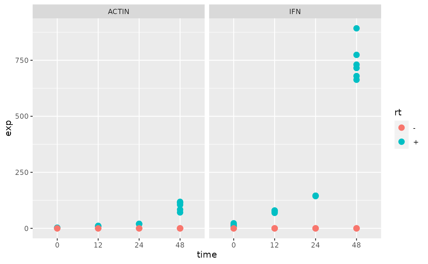
#> 16 wt     IFN   48      780.   9633

Plots

Plot the expression for each gene over time.
Calculate a fold-change for IFN over ACTIN and re-plot.

Exercises

Tidy the mtcars data set. Note that car names are rownames in the built-in data, so they need to be moved to their own column prior to tibble conversion. You can use tibble:rownames_to_column() for this purpose.

The tidied data should look something like:

#> # A tibble: 352 × 3
#>    name              var   value
#>    <chr>             <chr> <dbl>
#>  1 Mazda RX4         mpg    21  
#>  2 Mazda RX4 Wag     mpg    21  
#>  3 Datsun 710        mpg    22.8
#>  4 Hornet 4 Drive    mpg    21.4
#>  5 Hornet Sportabout mpg    18.7
#>  6 Valiant           mpg    18.1
#>  7 Duster 360        mpg    14.3
#>  8 Merc 240D         mpg    24.4
#>  9 Merc 230          mpg    22.8
#> 10 Merc 280          mpg    19.2
#> # … with 342 more rows

For each car in the tidy mtcars data set, calculate the mean (mean()) and variance (var()) for each variable. Try using summarize(), and summarize_at() or summarize_all().
Plot mpg vs cyl for the mtcars data set. Which format should you use? The original data set, or the tidied one? Why?
Using the provided qpcr data, plot the changes in gene expression over time. Use colors to represent genotypes and facets for the different genes. If that’s too easy, add error bars (geom_errorbar()) and connect each point with a line (geom_line()).

Too Easy?

If you found those exercises too easy, try these:

Tidy the anscombe data set. Your tidy data should look like:

# A tibble: 44 x 3
   set       x     y
   <chr> <dbl> <dbl>
 1 1         4  4.26
 2 1         5  5.68
 3 1         6  7.24
 4 1         7  4.82
 5 1         8  6.95
 6 1         9  8.81
 7 1        10  8.04
 8 1        11  8.33
 9 1        12 10.8 
10 1        13  7.58
# ... with 34 more rows

Calculate summary statistics in your tidy anscombe data. Calculate n, mean, and var for each x and y variable in the sets. Try using summarize_each for this calculation.

Calculate the cor between x and y for each set. What do you infer from these summary statistics?

Plot the tidy anscombe data. Plot each x/y point on separate facets for each set, and plot a smoothing line. Examine the plots. How do they compare to the summary statistics?

ggplot(anscombe_tidy, aes(x, y)) +
  geom_point() +
  facet_wrap(~set) +
  geom_smooth(method = 'lm', se = FALSE)

Class 1: Course Overview | Data Import and Tidying

Jay Hesselberth

2022-07-06

Goals for the course

RStudio Overview

Environment

`read` functions

Console

Viewer

Editor

Projects

Tidyverse cheatsheets

Git and Github

Formatting data for efficient analysis

The `tibble`

The `tidyr` package

`gather` and `spread`

Long format

Wide format

Exercise

`separate` and `unite`

`separate`

`crossing` and `complete`

Data in the 96-well plate format.

Sample names

Extracting sample names

Data manipulation

qPCR data

qPCR data tidying

Sample names

Data joining

Statistical summary

Plots

Exercises

Too Easy?

Class 1: Course Overview | Data Import and Tidying

Jay Hesselberth

2022-07-06

Goals for the course

RStudio Overview

Environment

read functions

Console

Viewer

Editor

Projects

Tidyverse cheatsheets

Git and Github

Formatting data for efficient analysis

The tibble

The tidyr package

gather and spread

Long format

Wide format

Exercise

separate and unite

separate

crossing and complete

Data in the 96-well plate format.

Sample names

Extracting sample names

Data manipulation

qPCR data

qPCR data tidying

Sample names

Data joining

Statistical summary

Plots

Exercises

Too Easy?

`read` functions

The `tibble`

The `tidyr` package

`gather` and `spread`

`separate` and `unite`

`separate`

`crossing` and `complete`