Introduction to nihexporter • nihexporter

Abstract

The National Institutes of Health (NIH) is the major source of federal funding for biomedical research in the United States. Analysis of past and current NIH funding can illustrate funding trends and identify productive research topics, but these analyses are conducted ad hoc by the institutes themselves and only provide a small glimpse of the available data. The NIH provides free access to funding data via NIH EXPORTER, but few tools have been developed to enable analysis of these data.

We developed the nihexporter R package, which provides access to NIH EXPORTER data. We used the package to develop several analysis vignettes that show funding trends across NIH institutes over 15 years and highlight differences in how institutes change their funding profiles. Investigators and institutions can use the package to perform self-studies of their own NIH funding.

Introduction

The National Institutes of Health (NIH) is the major source federal funds for biomedical research in the United States. The NIH budget is approved by Congress each year. The NIH is divided into 25 institutes, each with its own focus and mission. For example, National Cancer Institue (NCI) focuses on malignant diseases; the National Institute for Allergy and Immune Disease focuses on the immune system and transmissible diseasei; and the National Institute for General Medical Sciences focuses on basic research, without a specific disease focus. Each institute negotiates with the NIH director for its yearly budget, with budget institutes ranging from millions to several billion dollars.

The NIH provides funds through competitive grants written by internal and external investigators, and the funds associated with these grants can be divided into ‘direct’ and ‘indirect’ costs. Direct costs are funds that are given to an investigator (or group of investigators) to conduct their proposed research. These funds buy supplies for the experiments and pay the salaries of people to do the work.

By contrast, indirect costs are funds that are paid to institutions associated with investigators, and are used to “keep the lights on”: they pay for infrastructure costs. However, the “indirect cost recovery” (ICR) rate of each institution, the fraction of each award the institute receives, is congressionally mandated, and there is a wide range in ICR rates. Some of the highest ICR rates are close to 100%, meaning that for every dollar an investigator receives, the institutions receive an equal amount.

NIH funding is an investment strategy: the institutes invest money in specific research areas, hoping for future returns in the form of publications, patents and skilled trainees. As with any investment strategy, a periodic review can help rebalance the portfolio in order to maximize returns. Analysis of NIH funding data has been performed internally by the NIH, or by contracted third-parties. Several of these analyses have highlighted funding trends and suggested metrics to gauge the ‘return’ on the NIH ‘investment’. For example, “productivity” can be examined as a function of the number of publications produced by grants per dollar of “direct costs”.

Methods

We downloaded NIH funding data from the NIH EXPORTER website in comma-separated value (CSV) format and parsed these data into R data files that each contain specific information:

projects has information about projects in each fiscal year, keyed by project.num
project_pis links PI information to a project
publinks table links PubMed IDs to project.num
publications links project IDs to PubMed IDs
patents links patent IDs to project IDs

See the documentation in the R package for more information about each table.

The package also has several precomputed variables and tables that enable quick and easy exploratory analysis:

nih_institutes: Two-letter format for 27 NIH institutes
project_io: This table contains pre-computed values for overall project cost (project_cost), as well as the number of publications (n_pubs) and patents (n_patents) associated with each project.

NIH EXPORTER provides access to the total costs of each grant in each fiscal year, comprising both direct and indirect costs.

Results and Discussion

Project costs

Let’s look at the costs of grants over time for a few institutes:

library(nihexporter)
library(tidyverse)
library(cowplot)
library(DT)

select_inst <- c('GM', 'AI', 'CA')
cost.over.time <- projects |>
  select(institute, fy_cost, fiscal_year) |>
  filter(institute %in% select_inst) |>
  summarize(
    yearly_cost = sum(fy_cost, na.rm = TRUE),
    .by= c(fiscal_year, institute)
  )

ggplot(
  cost.over.time,
  aes(
    x = factor(fiscal_year), 
    y = yearly_cost / 1e9,
    group = institute,
    color = institute
  )
) +
  geom_line() +
  geom_point() +
  theme_cowplot() +
  theme(legend.position = 'top') +
  labs(
    title = 'Institute spending, FY 2000-2021',
    x = 'Fiscal year',
    y = 'Project costs (USD, billions)'
  ) +
  scale_color_brewer(palette = 'Dark2') +
  scale_x_discrete(guide = guide_axis(angle = 45))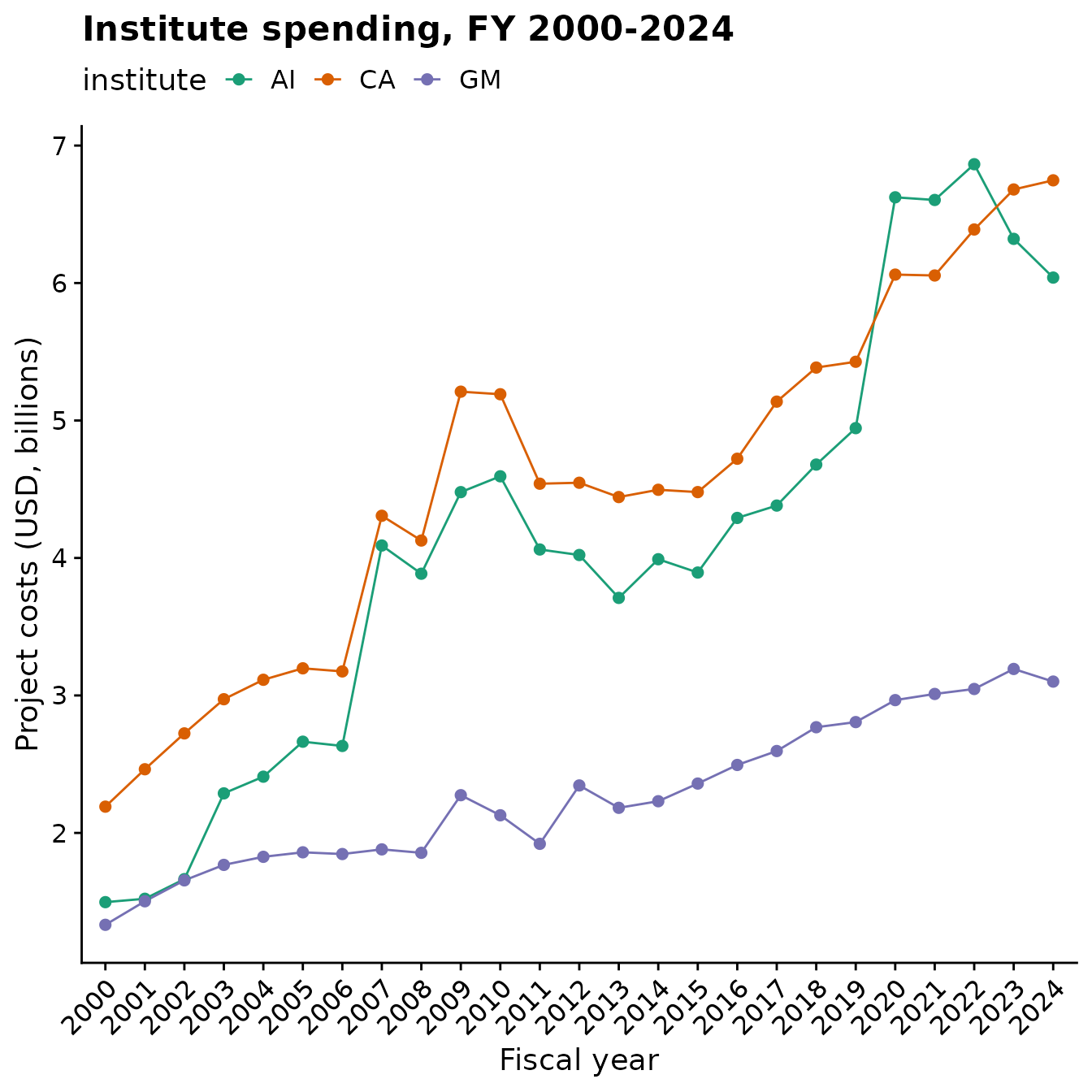

Funding distributions

By Institution

Let’s look where the money is going.

institution_funding <- projects |>
  filter(activity == 'R01') |>
  summarise(
    total_dollars = sum(fy_cost, na.rm = TRUE),
    .by = c(org_name, fiscal_year)
    ) |>
  arrange(desc(total_dollars))

institution_funding |>
  mutate(total_dollars = total_dollars / 1e6) |>
  datatable(
    caption='R01 grant dollars awarded to specific institutions',
    colnames=c('Org', 'Fiscal year', 'Dollars (millions)')
  )

By PI

One can also examine how dollars are accrued by specific PIs. It is not possible to assign dollars directly to a PI, because some grants have multiple investigators. Rather, these are total costs that a given PI has been associated with over all grants in NIH EXPORTER. Here we identify PIs with the largest dollar amounts accrued for R01 grants.

pi_funding_r01 <- projects |>
  filter(activity == 'R01') |>
  left_join(project_io, by = 'project_num') |>
  left_join(project_pis, by = 'project_num') |>
  filter(!is.na(pi_id)) |>
  select(project_num, pi_id, total_cost) |> 
  summarise(
    pi_funding = sum(total_cost) / 1e6,
    .by = (pi_id)
    ) |>
  arrange(desc(pi_funding))  

pi_funding_r01 |>
  datatable(
    caption = 'R01 funding associated with specific PIs',
    colnames=c('PI ID', 'USD, millions')
  )

Productivity

To measure the return on the NIH investment, we can measure scholarly output (i.e., publications) per dollar invested.

Here we identify th highest performing grants outside of the R01 category. Much has been made of the wasteful spending outside of investigator-initiated research. Here we identify the cost of publications for grants other than R01s.

high_perf_not_r01 <- projects |>
  filter(activity != 'R01') |>
  left_join(project_io, by = 'project_num') |>
  select(project_num, total_cost, n_pubs) |>
  filter(total_cost > 1e6 & n_pubs > 0) |>
  mutate(cost_per_pub = round(total_cost / n_pubs / 1e3, 3)) |>
  arrange(cost_per_pub)

high_perf_not_r01 |>
  head(10) |>
  mutate(
    total_cost = round(total_cost / 1e6, 3),
    ) |>
  datatable(
    caption = 'Productivity (publications / dollar) of non-R01 grants',
    colnames = c(
      'Project ID', 'Project cost (USD, millions)',
      'Number of publications', 'Cost per publications (USD, thousands)'
    )
  )

We can also identify the specific publications associated with grants with the least expensive publications.

high_perf_not_r01 |>
  head(1) |>
  select(project_num) |>
  left_join(publinks, by = 'project_num') |>
  datatable(
    caption='Publications from the most productive grants',
    colnames=c('Project ID', 'Pubmed ID')
  )

We can also identify productive PIs with current R01s …

productive_pis <- projects |>
  filter(activity == 'R01') |>
  select(project_num) |>
  left_join(project_io, by = 'project_num') |>
  left_join(project_pis, by = 'project_num') |>
  summarize(
    total_pi_funding = sum(total_cost, na.rm = TRUE),
    total_pubs = sum(n_pubs),
    .by = c(pi_id)
    ) |>
  mutate(
    pub_cost = total_pi_funding / total_pubs
    ) |>
  # prevent PI Ids from being commafied
  mutate(pi_id = as.character(pi_id)) |>
  arrange(pub_cost)

productive_pis |>
  head(100) |>
  datatable(
    caption='Publications from the most productive grants',
    colnames = c(
      'PI ID',
      'Cost per publication (USD)',
      'Total publications',
      'Total project costs (USD)'
    )
  )

Or we can identify the all-time most produtive PIs, independent of grant type or time frame …

productive_pis_all_time <- projects |>
  select(project_num, activity) |>
  left_join(project_io, by = 'project_num') |>
  left_join(project_pis, by = 'project_num') |>
  summarize(
    total_pi_dollars = sum(total_cost, na.rm = TRUE),
    total_pubs = sum(n_pubs),
    total_patents = sum(n_patents),
    .by = c(pi_id, activity)
    ) |>
  filter(total_pi_dollars >= 1e6) |>
  mutate(
    pub_cost = total_pi_dollars / total_pubs,
    patent_cost = total_pi_dollars / total_patents
    ) |>
  select(
    pi_id, activity, pub_cost, patent_cost, 
    total_pubs, total_patents, total_pi_dollars
  )

productive_pis_all_time |>
  select(-patent_cost, -total_patents) |>
  arrange(pub_cost) |>
  head(10) |>
  DT::datatable(
    caption = 'Most productive PIs all time for publications',
    colnames = c(
      'PI ID', 'Grant type',
      'Cost per publication (dollars)',
      'Total publications',
      'Total dollars')
  )

productive_pis_all_time |> select(-pub_cost, -total_pubs) |> arrange(patent_cost) |> head(10) |> DT::datatable( caption = 'Most productive PIs all time for patents', colnames = c( 'PI ID', 'Grant type', 'Cost per patent (dollars)', 'Total patents', 'Total dollars' ) )

When Jeremy Berg was head of the Institute of General Medical Sciences (NIGMS) from 2003-2011, he routinely provided analysis of funding trends at NIGMS in his “Feedback Loop” blog. One of these measured the productivity per grant dollar by measuring its “scholarly output” (i.e., publications) as a function of direct costs. In this plot there is an increase in productivity per dollar, until an inflection point at $700K, after which the number of publications drops, suggesting a negative influence of grant money on scholarly output. This was interesting and covered here.

Here we flesh out this analysis and look at how all institutes perform by this measure (Berg, and now Lorsch, only analyzed GM). One caveat is that we only have access to total.cost in NIH EXPORTER, so the numbers include indirect costs. But, this is real cost to the tax-payer.

First, we need to calculate the lifetime costs of all R01 grants.

# calculate costs of all grants, over the entire lifetime of the grant
grant_costs <- projects |>
  filter(institute %in% nih_institutes & activity == 'R01') |>
  left_join(project_io, by = 'project_num') |>
  select(institute, project_num, total_cost, n_pubs) |>
  unique()

grant_costs
#> # A tibble: 116,579 × 4
#>    institute project_num total_cost n_pubs
#>    <fct>     <chr>            <dbl>  <int>
#>  1 AA        R01AA000187     192057     67
#>  2 AA        R01AA000279    1368179      6
#>  3 AA        R01AA000626    4256757    118
#>  4 AA        R01AA002666    2635998    171
#>  5 AA        R01AA002686    9560051     73
#>  6 AA        R01AA003037     710028     16
#>  7 AA        R01AA003490    2285856     33
#>  8 AA        R01AA003972    2695918     58
#>  9 AA        R01AA004610    5035947     39
#> 10 AA        R01AA004961     477993     76
#> # ℹ 116,569 more rows

Next, we need to identify grants in each of the bins that Berg previously alluded to. dplyr makes this easy with the ntile() function. Berg previously divided grants into ~15 bins, we’ll bin into ~5%.

bin_grant_costs <- grant_costs |>
  group_by(institute) |>
  group_by(n_tile = ntile(total_cost, 20)) 

bin_grant_costs
#> # A tibble: 116,579 × 5
#> # Groups:   n_tile [20]
#>    institute project_num total_cost n_pubs n_tile
#>    <fct>     <chr>            <dbl>  <int>  <int>
#>  1 AA        R01AA000187     192057     67      1
#>  2 AA        R01AA000279    1368179      6      8
#>  3 AA        R01AA000626    4256757    118     19
#>  4 AA        R01AA002666    2635998    171     16
#>  5 AA        R01AA002686    9560051     73     20
#>  6 AA        R01AA003037     710028     16      3
#>  7 AA        R01AA003490    2285856     33     15
#>  8 AA        R01AA003972    2695918     58     16
#>  9 AA        R01AA004610    5035947     39     20
#> 10 AA        R01AA004961     477993     76      2
#> # ℹ 116,569 more rows

# Berg's original values ...
# breaks <- c(175000, 200000, 225000, 250000, 300000, 375000, 400000,
#           450000, 500000, 600000, 700000, 800000, 900000, 1000000)
min.lifetime.cost <- round(min(grant_costs$total_cost, na.rm = TRUE), -4) # round to 10,000s
max.lifetime.cost <- round(max(grant_costs$total_cost, na.rm = TRUE), -5) 
# step is average size of an award
step <- 1e6

breaks <- seq(min.lifetime.cost, max.lifetime.cost, step)
breaks
#>   [1] 0.00e+00 1.00e+06 2.00e+06 3.00e+06 4.00e+06 5.00e+06 6.00e+06
#>   [8] 7.00e+06 8.00e+06 9.00e+06 1.00e+07 1.10e+07 1.20e+07 1.30e+07
#>  [15] 1.40e+07 1.50e+07 1.60e+07 1.70e+07 1.80e+07 1.90e+07 2.00e+07
#>  [22] 2.10e+07 2.20e+07 2.30e+07 2.40e+07 2.50e+07 2.60e+07 2.70e+07
#>  [29] 2.80e+07 2.90e+07 3.00e+07 3.10e+07 3.20e+07 3.30e+07 3.40e+07
#>  [36] 3.50e+07 3.60e+07 3.70e+07 3.80e+07 3.90e+07 4.00e+07 4.10e+07
#>  [43] 4.20e+07 4.30e+07 4.40e+07 4.50e+07 4.60e+07 4.70e+07 4.80e+07
#>  [50] 4.90e+07 5.00e+07 5.10e+07 5.20e+07 5.30e+07 5.40e+07 5.50e+07
#>  [57] 5.60e+07 5.70e+07 5.80e+07 5.90e+07 6.00e+07 6.10e+07 6.20e+07
#>  [64] 6.30e+07 6.40e+07 6.50e+07 6.60e+07 6.70e+07 6.80e+07 6.90e+07
#>  [71] 7.00e+07 7.10e+07 7.20e+07 7.30e+07 7.40e+07 7.50e+07 7.60e+07
#>  [78] 7.70e+07 7.80e+07 7.90e+07 8.00e+07 8.10e+07 8.20e+07 8.30e+07
#>  [85] 8.40e+07 8.50e+07 8.60e+07 8.70e+07 8.80e+07 8.90e+07 9.00e+07
#>  [92] 9.10e+07 9.20e+07 9.30e+07 9.40e+07 9.50e+07 9.60e+07 9.70e+07
#>  [99] 9.80e+07 9.90e+07 1.00e+08 1.01e+08 1.02e+08 1.03e+08 1.04e+08
#> [106] 1.05e+08 1.06e+08 1.07e+08 1.08e+08 1.09e+08 1.10e+08 1.11e+08
#> [113] 1.12e+08 1.13e+08 1.14e+08 1.15e+08

dollar_bin_grant_costs <- grant_costs |>
  mutate(
    dollar.tile = findInterval(
      total_cost, vec = breaks, 
      all.inside = TRUE, rightmost.closed = TRUE
    ),
    .by = institute
  )

dollar_bin_grant_costs
#> # A tibble: 116,579 × 5
#>    institute project_num total_cost n_pubs dollar.tile
#>    <fct>     <chr>            <dbl>  <int>       <int>
#>  1 AA        R01AA000187     192057     67           1
#>  2 AA        R01AA000279    1368179      6           2
#>  3 AA        R01AA000626    4256757    118           5
#>  4 AA        R01AA002666    2635998    171           3
#>  5 AA        R01AA002686    9560051     73          10
#>  6 AA        R01AA003037     710028     16           1
#>  7 AA        R01AA003490    2285856     33           3
#>  8 AA        R01AA003972    2695918     58           3
#>  9 AA        R01AA004610    5035947     39           6
#> 10 AA        R01AA004961     477993     76           1
#> # ℹ 116,569 more rows

dollar_bin_grant_costs |> summarize(count = n(), .by = dollar.tile)
#> # A tibble: 44 × 2
#>    dollar.tile count
#>          <int> <int>
#>  1           1 25143
#>  2           2 50436
#>  3           5  4061
#>  4           3 21171
#>  5          10   232
#>  6           6  2297
#>  7           4 10444
#>  8           9   357
#>  9           7  1290
#> 10           8   659
#> # ℹ 34 more rows

That looks better. Now we can make the summary plots …

ggplot(
  # need to remove higher tiles because there are too few grants
  filter(dollar_bin_grant_costs, dollar.tile <= 13),
  aes(
    x = factor(dollar.tile),
    y = n_pubs
  )
) +
  geom_boxplot(
    color = 'grey50',
    fill = 'red',
    alpha = 0.1,
    outlier.shape = NA
    ) +
  scale_x_discrete(labels = breaks / 1e6) + 
  theme(
    axis.text.x = element_text(angle=45, vjust=0.8)
    ) + 
  scale_y_log10() +
  theme_cowplot() +
  facet_wrap(~ institute, scales = "free_x") +
  labs(
    y = 'Number of publications',
    x = 'Total costs (minimum, in millions USD)'
  )

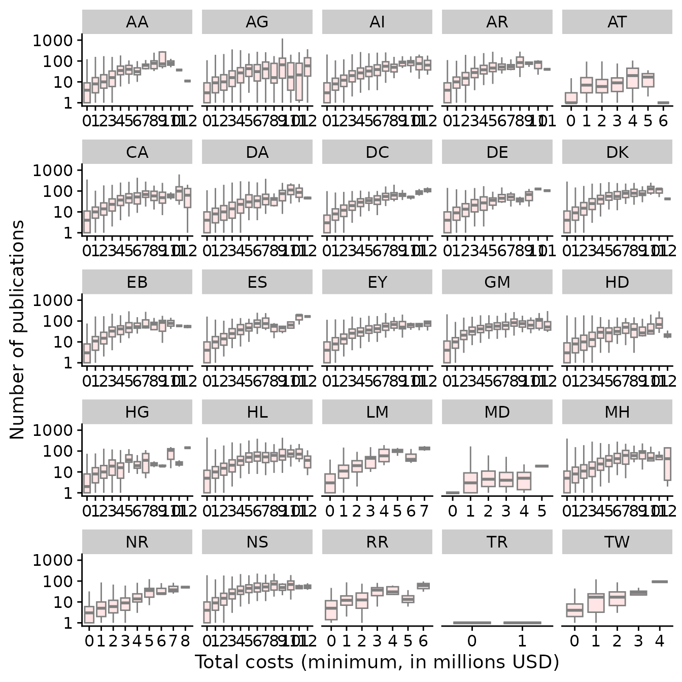
Productivity versus grant costs for each institute.

Comparison of grant programs

The NIH provides funds through differet grant programs:

research: investigator-intitiated, actvities begin with R (e.g., R01)
program: activities begin with P (e.g. P01)
cooperative agreements: actvities begin with U (e.g. U54)

We can examine the total costs spent on specific grants and specific institutes over time.

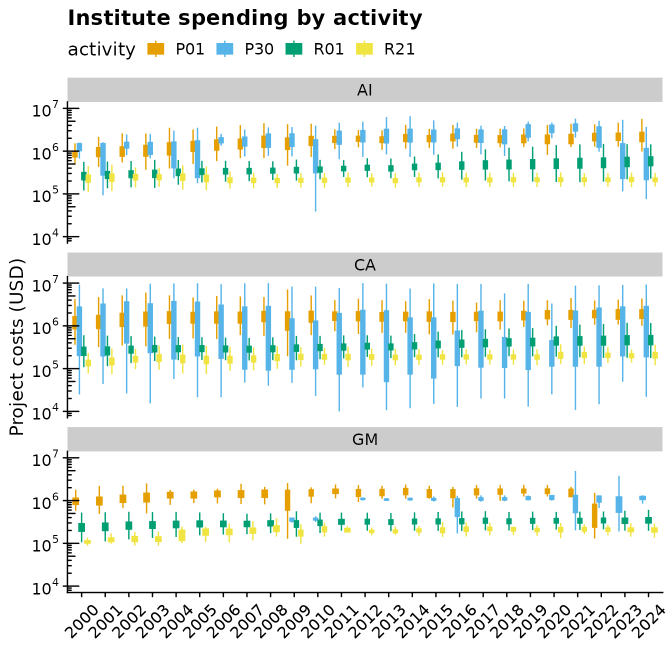
Funds for specific types of grants at the GM, CA and AI institutes

Or we can see how institutes allocate money generally to different types of grants.


# from https://grants.nih.gov/grants/funding/funding_program.htm
research_projects <- projects |> filter(grepl('^R', activity)) |> select(project_num)
program_projects <- projects |> filter(grepl('^P', activity)) |> select(project_num)
coop_projects <- projects |> filter(grepl('^U', activity)) |> select(project_num)

select_inst <- c('AI','CA','GM','HG','AA','MH')
                
grant_costs <- projects |>
  filter(institute %in% select_inst) |>
  select(project_num, institute, fiscal_year, fy_cost)

research_costs <- grant_costs |>
  semi_join(research_projects, by = 'project_num') |>
  summarize(
    project_cost = sum(fy_cost, na.rm = TRUE),
    .by = c(project_num, institute, fiscal_year)
    ) |>
  mutate(type = 'research')

program_costs <- grant_costs |>
  semi_join(program_projects, by = 'project_num') |>
  summarize(
    project_cost = sum(fy_cost, na.rm = TRUE),
    .by = c(project_num, institute, fiscal_year)
    ) |>
  mutate(type = 'program')

coop_costs <- grant_costs |>
  semi_join(coop_projects, by = 'project_num') |>
  summarize(
    project_cost = sum(fy_cost, na.rm = TRUE),
    .by = c(project_num, institute, fiscal_year)
    ) |>
  mutate(type = 'cooperative agreements')

combined_tbl <- bind_rows(research_costs, program_costs, coop_costs)

ggplot(
  combined_tbl,
  aes(
    x = factor(fiscal_year),
    y = project_cost,
    fill = type
    )
  ) +
  geom_boxplot(outlier.shape = NA) + 
  scale_y_log10(
    limits = c(1e4,1e7),
    labels = scales::trans_format("log10", scales::math_format(10^.x))
    ) +
  facet_wrap(~institute) +
  theme_cowplot() +
  scale_fill_brewer(palette = "Dark2") + 
  theme(legend.position = 'top') +
  labs(
    x = '',
    y = 'Total costs, log-scaled',
    title = 'Institute spencing by award type'
  ) +
  theme(
    axis.text.x = element_text(angle = 45, vjust = 0.5, hjust = 0.5)
  )

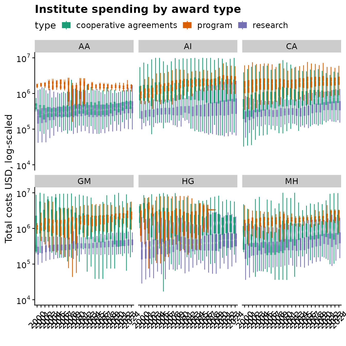
Comparison of research, program and coop costs over time

Duration

nihexporter exposes project.start and project.end, which we can use to examine the duration of projects. For example, we can identify the longest running R01 grants.

long_grants <- projects |>
  filter(activity == 'R01') |>
  select(project_num, project_start, project_end) |>
  group_by(project_num) |>
  summarize(
    longest_run = max(project_end, na.rm = TRUE) - min(project_start, na.rm = TRUE)) |>
  arrange(desc(longest_run)) |>
  mutate(in_years = round(as.numeric(longest_run) / 365), 3) |>
  select(project_num, in_years)

long_grants |>
  head(1000) |>
  DT::datatable(
    caption = 'Longest running R01 grants (all-time)',
    colnames=c('Project ID', 'Duration (years)')
  )

Geographical distribution

Geographical distribution of grant dollar is easily visualized using the package.

state_data <- data.frame(org_state = state.abb,
                         state_name = tolower(state.name))

state_funding <- projects |>
  select(application_id, org_state, fy_cost) |>
  group_by(org_state) |>
  summarize(total_fy_cost = sum(fy_cost) / 1e9)

cost_by_state <- state_funding |>
  left_join(state_data) |>
  select(state_name, total_fy_cost) |>
  filter(state_name != "NA") |>
  mutate(region=state_name, cost = total_fy_cost) |>
  select(region, cost)

state_map_data <- map_data("state")

plot_data <- left_join(state_map_data, cost_by_state)

ggplot() + 
  geom_polygon(
    data=plot_data, 
    aes(x=long, y=lat, group = group, fill=plot_data$cost),
    colour="black"
    ) +
  scale_fill_continuous(low = "lightgrey", high = "red", guide="colorbar") +
  theme_bw() +
  labs(fill = "Total Cost per year \n (USD, billions)",x="", y="") +
  scale_y_continuous(breaks=c()) +
  scale_x_continuous(breaks=c()) +
  theme(panel.border =  element_blank()) +
  coord_fixed(ratio = 1.4)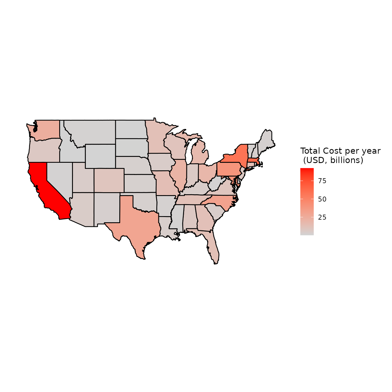

Geographic distribution of NIH dollars