aRt competition entries

Vote for your favorites at this Google Form.

Plot 1

Code

library(tidyverse)
library(patchwork)
library(emo)

# need length.out and sequence function to have enough data points to make smooth curved lines; here I create a tbl with values for theta and a corresponding r for my coordinate plot
tbl <- tibble(
  theta = seq(0, 2 * 3.14, length.out = 500),
  r = (3 * sin(pi * theta))
)

# create a plot of each coordinate point and changed the aesthetics to adjust x and y to make an abstract plot. With different variations I came upon these aesthetic adjustments to create what looks like a squid
ggplot(tbl) +
  geom_point(
    aes(x = r * theta, y = r^2),
    color = "#613092",
    alpha = 0.75,
    size = 0.25
  ) +
  coord_polar(start = 0) +
  #added a face to my squid using annotate
  annotate(
    "text",
    x = 0,
    y = -4,
    label = "❁´◡`❁  ",
    size = 7,
    color = "#452268",
    angle = 4
  ) +

  # added a title amd subtitle
  labs(
    title = "Hugs From Miss Squid",
    subtitle = "❤️  ❤️  ❤️ ❤️ ❤️ ❤️ ❤️ ❤️ ❤️ ❤️ ❤️"
  ) +
  theme(
    plot.subtitle = element_text(color = "red")
  ) +

  # used theme_void() to remove the coordinate plot background and axis labels so I was left with a white background behind my data points (squid body) and annotated text (face of squid)
  theme_void()

Plot 2

Code

library(ggplot2)
library(dplyr)
library(viridis)

set.seed(42)
x <- seq(-4 * pi, 4 * pi, length.out = 2000)

# Mountain Layers
mountain_data <- data.frame(
  x = rep(x, 5),
  layer = rep(1:5, each = length(x))
) %>%
  mutate(
    # Base mountain shape
    base_height = case_when(
      layer == 1 ~ 3 * sin(x / 2) + 1.5 * sin(x / 1.3) + 0.8 * sin(x * 0.7),
      layer == 2 ~ 2.5 * sin(x / 1.8) + 1.2 * sin(x / 1.1) + 0.6 * sin(x * 0.9),
      layer == 3 ~ 2 * sin(x / 2.2) + sin(x / 0.9) + 0.4 * sin(x * 1.2),
      layer == 4 ~ 1.5 * sin(x / 2.8) + 0.8 * sin(x / 1.5) + 0.3 * sin(x * 1.5),
      layer == 5 ~ sin(x / 3.2) + 0.5 * sin(x / 2.1) + 0.2 * sin(x * 1.8)
    ),
    # Noise for texture
    noise = rnorm(n(), 0, 0.1 * (6 - layer)),
    y = pmax(base_height + noise, -layer * 0.5), # Ensure layers don't go below each other
    # Color based on height and layer for atmospheric perspective
    fill_color = layer + (y - min(y)) / (max(y) - min(y))
  )

# Plot each layer
p1 <- ggplot() +
  # Layer 5 (background)
  geom_ribbon(
    data = filter(mountain_data, layer == 5),
    aes(x = x, ymin = -2.5, ymax = y),
    fill = "#440154",
    alpha = 0.6
  ) +
  # Layer 4
  geom_ribbon(
    data = filter(mountain_data, layer == 4),
    aes(x = x, ymin = -2, ymax = y),
    fill = "#31688e",
    alpha = 0.7
  ) +
  # Layer 3
  geom_ribbon(
    data = filter(mountain_data, layer == 3),
    aes(x = x, ymin = -1.5, ymax = y),
    fill = "#26828e",
    alpha = 0.75
  ) +
  # Layer 2
  geom_ribbon(
    data = filter(mountain_data, layer == 2),
    aes(x = x, ymin = -1, ymax = y),
    fill = "#35b779",
    alpha = 0.8
  ) +
  # Layer 1 (foreground)
  geom_ribbon(
    data = filter(mountain_data, layer == 1),
    aes(x = x, ymin = -0.5, ymax = y),
    fill = "#fde725",
    alpha = 0.85
  ) +
  labs(title = "The Rocky Mountains", x = "", y = "") +
  theme_void() +
  theme(
    plot.background = element_rect(fill = "black", color = NA),
    panel.background = element_rect(fill = "black", color = NA),
    plot.title = element_text(color = "white", size = 16, hjust = 0.5),
    plot.subtitle = element_text(color = "white", size = 12, hjust = 0.5),
    legend.position = "none"
  )

print(p1)

Plot 3

Code

# aRt Title: Transcript City

# Use transcriptomic data from ps-04.
# Select for gene name & RNA_fc values only.
# Drop NAs & remove duplicates.
# Filter rna_fc within a positive range that is reasonable to display.

library(tidyverse)
library(here)

art_tbl <- read_csv(
  here("data/bootcamp/data_rna_protein.csv.gz")
)

art_tbl_trim <- art_tbl |>
  select(gene = geneid, rna_fc = iDUX4_logFC) |>
  drop_na() |>
  distinct(gene, .keep_all = TRUE) |>
  filter(rna_fc > 0 & rna_fc <= 0.5) |>
  # Mutate to assign `color_class` based on arbitrary rna_fc value; will be used to vary color in plot
  mutate(
    color_class = case_when(
      rna_fc < 0.1 ~ "A",
      rna_fc < 0.2 ~ "B",
      rna_fc < 0.3 ~ "C",
      rna_fc < 0.4 ~ "D",
      .default = "E"
    )
  ) |>
  # Mutate to assign `star_class` based on first letter of gene name. Use this stackoverflow post to understand partial strings: https://stackoverflow.com/questions/56993566/how-to-create-a-new-column-based-on-partial-string-of-another-column
  mutate(
    star_class = substr(gene, 1L, 1L)
  )

city_palette <- c("#eeaf61", "#fb9062", "#ee5d6c", "#ce4993", "#6a0d83")

ggplot(
  art_tbl_trim,
  aes(
    x = gene,
    y = rna_fc,
    fill = color_class
  )
) +
  geom_col() +
  geom_point(
    shape = 8,
    color = "white",
    size = 0.2
  ) +
  theme(
    # Remove legend, axis titles, grid, & make background black
    legend.position = "none",
    axis.title = element_blank(),
    axis.text = element_blank(),
    axis.ticks = element_blank(),
    panel.grid = element_blank(),
    panel.background = element_rect(fill = 'black')
  ) +
  scale_fill_manual(values = city_palette)

Plot 4

Code

library(ggplot2)

pride_colors <- c(
  "maroon",
  "purple",
  "pink",
  "lavender",
  "steelblue",
  "turquoise",
  "springgreen",
  "snow4"
)

stripes_df <- data.frame(
  ymin = seq(0, 7),
  #Ymin needs to match the number of colors you've picked out
  ymax = seq(1, 8),
  #Ymax is setting the width of each rectangle to be 1 unit later on
  color = pride_colors
)

base_flag <- ggplot(stripes_df) +
  geom_rect(
    aes(xmin = 0, xmax = 15, ymin = ymin, ymax = ymax, fill = color),
    color = NA
  )

#Create a triangle polygon df

triangle_df <- data.frame(
  x = c(0, 0, 5),
  y = c(0, 8, 4) # bottom, top, center
)

combined_flag <- base_flag +
  geom_polygon(
    data = triangle_df,
    aes(x = x, y = y),
    fill = "orange",
    alpha = 0.7
  ) +
  scale_fill_identity() +
  theme_void() +
  coord_fixed()

dots_df <- data.frame(
  x = runif(400, 0, 15), # Random x across flag width
  y = runif(400, 0, length(pride_colors)), # Random y across flag height
  size = runif(400, 0.5, 2), # Dot sizes
  alpha = runif(400, 0.1, 0.4), # Transparency
  color = sample(pride_colors, 400, replace = TRUE) # Pride color for each dot
)

# Final plot
combined_flag +
  geom_point(
    data = dots_df,
    aes(x = x, y = y, size = size, alpha = 0.7, color = color),
    show.legend = FALSE
  ) +
  #scale_fill_identity() +
  theme_void() +
  coord_fixed()

Plot 5

Code

library(tidyverse)
data("trees")
trees_tibble <- as_tibble(trees)

ggplot_trees <- ggplot(
  data = trees_tibble,
  mapping = aes(
    x = Girth,
    y = Height,
    size = Volume
  )
) +
  geom_point(
    alpha = 1.0,
    shape = 8,
    color = "#FF0000",
    size = 10,
    stroke = 1
  ) +
  geom_smooth(
    alpha = 0.5,
    color = "#0000FF",
    fill = "#8A00C4",
    linetype = "dashed",
    size = 3
  ) +
  theme(
    plot.background = element_rect(fill = "#FFFF00"),
    panel.background = element_rect(fill = "#39FF14"),
    panel.grid.major = element_line(color = "#FF0000"),
    panel.grid.minor.x = element_line(color = "#0000FF"),
    panel.grid.minor.y = element_line(color = "#FFAE42"),
    panel.grid.major.y = element_line(color = "#FF13F0")
  ) +
  labs(
    x = "how thick is it (in) ??",
    y = "vertical dominance (ft)",
    title = "cool facts about 31 black cherry trees"
  )

ggplot_trees

Plot 6

Code

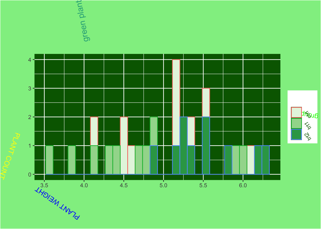
#generating histogram with labels and title
ugly_plant <- ggplot(PlantGrowth, aes(weight, fill = group, color = group)) +
  geom_histogram() +
  labs(x = "PLANT WEIGHT", y = "PLANT COUNT", title = "green plants")

#Theme changes for colors and position/angle of labels
ugly_plant +
  theme(
    plot.background = element_rect(fill = "lightgreen"),
    panel.background = element_rect(fill = "darkgreen"),
    panel.grid.major = element_line(colour = "white"),
    plot.title = element_text(color = "#29AB87", angle = 100, hjust = 6),
    axis.title.x = element_text(
      color = "blue",
      angle = 145,
      hjust = 1,
      vjust = 1
    ),
    axis.title.y = element_text(
      color = "yellow",
      angle = 250,
      hjust = 1,
      vjust = 1
    ),
    legend.title = element_text(
      color = "green",
      angle = 170,
      hjust = -1,
      vjust = -1
    ),
    legend.text = element_text(color = "darkgreen", angle = 120)
  ) +
  scale_fill_brewer(palette = "Light1")

Plot 7

Code

library(tidyverse)
library(here)
library(gganimate)
library(ragg)

storms_sin <- storms |> drop_na()

anim <- ggplot(
  storms_sin,
  aes(
    x = cos(pressure),
    y = sin(wind),
  )
) +
  geom_point(alpha = 0.05, shape = 11, size = 8, color = "#edf8b1") +
  theme_void() +
  coord_flip() +
  geom_point(
    aes(x = cos(pressure), y = sin(lat)),
    alpha = 0.3,
    shape = 8,
    size = 15,
    color = "#7fcdbb"
  ) +
  geom_density_2d_filled(
    aes(x = cos(pressure), y = sin(lat)),
    alpha = 0.1,
    linewidth = 12,
    color = "violet"
  ) +

  theme(
    legend.position = "none",
    plot.background = element_rect(fill = "#91c7d8"),
    panel.background = element_rect(fill = "#9c8080")
  ) +
  transition_states(
    transition_length = 0,
    state_length = 0.001,
    year
  )

spacestorm_plot <- animate(
  anim,
  device = "ragg_png",
  renderer = gifski_renderer()
)

anim_save(
  filename = "spacestorm.gif",
  animation = spacestorm_plot,
  path = here("img")
)

Plot 8

Code

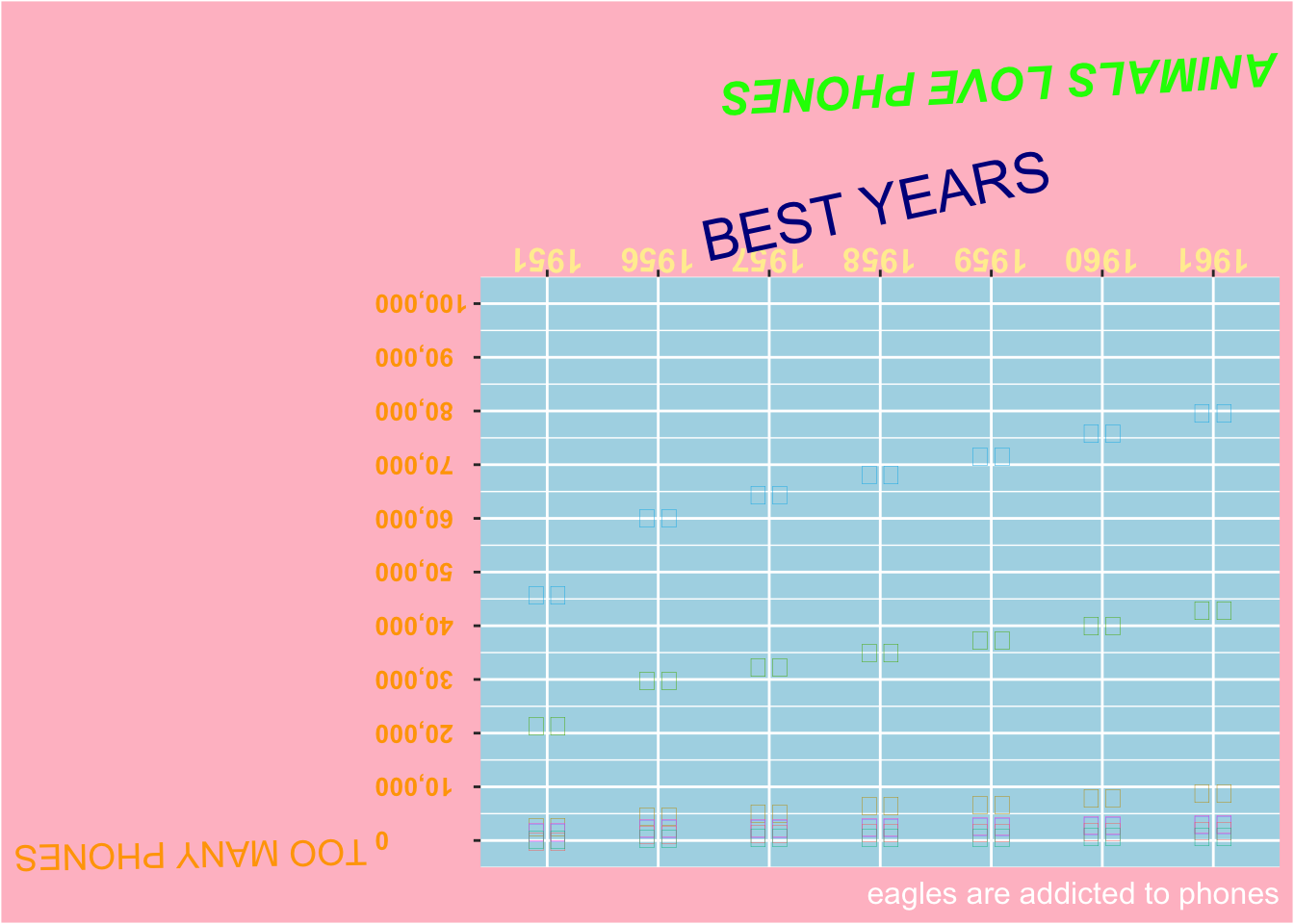
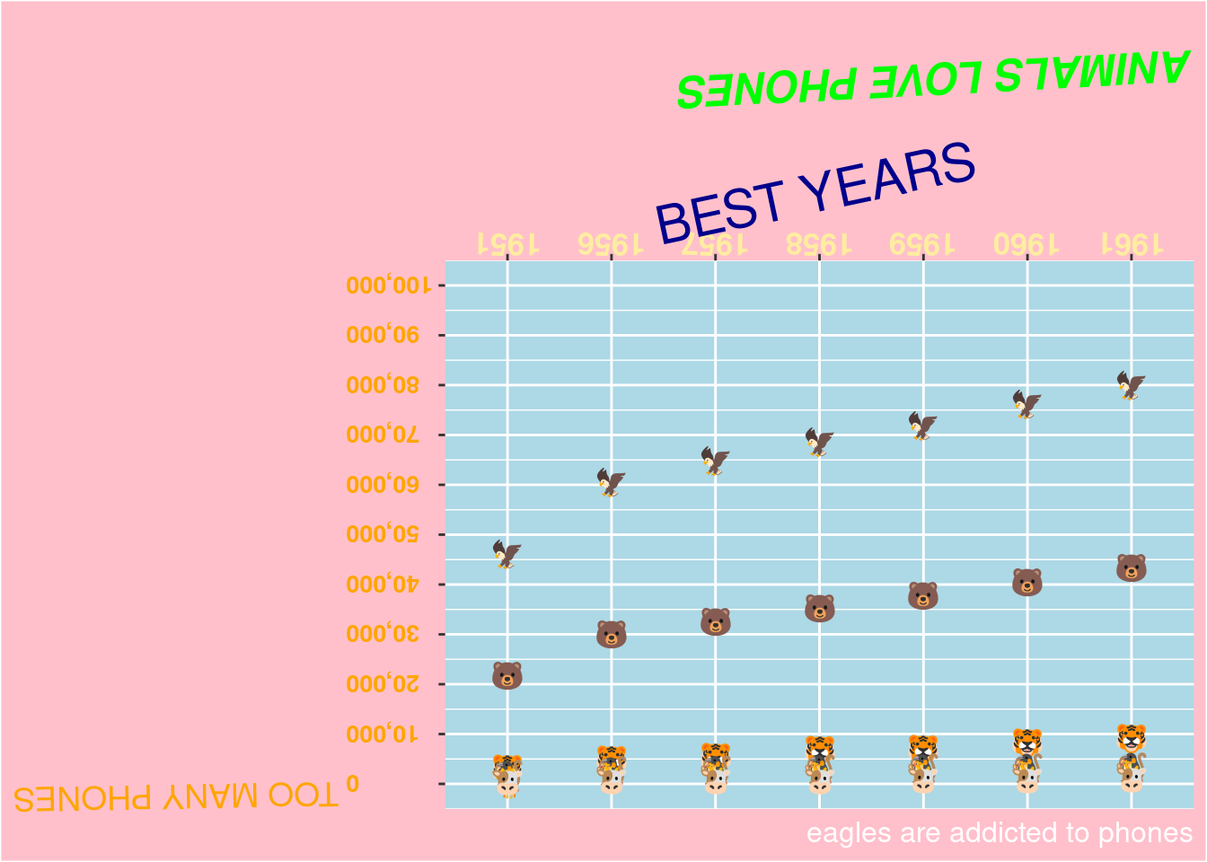
library(tidyverse)
library(emo)
# library(emojifont)
library(here)
library(gganimate)
library(ragg)
data("WorldPhones")

set.seed(42)

worldphones_tidy <- WorldPhones %>%
  as.data.frame() %>%
  rownames_to_column(var = "year") %>%
  pivot_longer(
    cols = -year,
    names_to = "region",
    values_to = "phones"
  ) %>%
  mutate(
    emoji = case_when(
      region == "N.Amer" ~ emo::ji("eagle"),
      region == "Europe" ~ emo::ji("bear"),
      region == "Asia" ~ emo::ji("tiger"),
      region == "S.Amer" ~ emo::ji("monkey"),
      region == "Oceania" ~ emo::ji("penguin"),
      region == "Africa" ~ emo::ji("giraffe"),
      region == "Mid.Amer" ~ emo::ji("cow")
    )
  ) %>%
  select(
    year,
    emoji,
    region,
    phones
  )

ggplot(
  worldphones_tidy,
  aes(
    x = year,
    y = phones,
    color = region
  )
) +
  geom_text(
    aes(label = emoji),
    size = 4,
    show.legend = FALSE
  ) +
  labs(
    x = "BEST YEARS",
    y = "TOO MANY PHONES",
    title = "ANIMALS LOVE PHONES",
    caption = "eagles are addicted to phones"
  ) +
  scale_y_continuous(
    limits = c(0, 100000),
    breaks = seq(0, 100000, 10000),
    labels = scales::comma
  ) +
  scale_x_discrete(position = "top") +
  theme(
    axis.text.x = element_text(
      face = "bold",
      color = "#ffeda0",
      size = 13,
      angle = 179
    ),
    axis.text.y = element_text(
      face = "bold",
      color = "orange",
      size = 10,
      angle = 180
    ),
    plot.background = element_rect(fill = "pink"),
    plot.title = element_text(
      face = "bold.italic",
      color = "green",
      size = 18,
      angle = 183
    ),
    plot.caption = element_text(color = "white", size = 12),
    axis.title.x = element_text(size = 22, color = "dark blue", angle = 12),
    axis.title.y = element_text(color = "orange", angle = 181, size = 14),
    panel.background = element_rect(fill = "light blue")
  )

Plot 9

Code

library(tidyverse)
library(here)
library(emo)
library(ggplot2)

exp_tbl <- read_csv(here("data/languages.csv"))

exp_tidy <-
  exp_tbl |>
  select(state, language, percent) |>
  drop_na()

ggplot(
  exp_tbl_tidy,
  aes(x = state, y = language, size = percent, color = percent)
) +
  geom_point(alpha = 0.50, fill = "tomato1", color = "red")
+labs(x = "States", y = "Language", title = "Linguistics")

Plot 10

Code

# Official ggplot for competition, emoji's where not working
emojimap <- c(
  "Tiger" = "🐆",
  "Cow" = "🐄",
  "African elephant" = "🐘",
  "Dog" = "🐕",
  "Goat" = "🐐",
  "Rabbit" = "🐇",
  "Pig" = "🐖",
  "Chimpanzee" = "🐒"
)

sleep_long <- msleep |>
  mutate(emoji = emojimap[name]) |>
  filter(!is.na(emoji)) |>
  select(emoji, name, brainwt, sleep_total, awake) |>
  drop_na() |>
  pivot_longer(
    c(sleep_total, awake),
    names_to = "state",
    values_to = "hours"
  ) |>
  mutate(
    factor(
      state,
      levels = c("awake", "sleep_total"),
      labels = c("Awake", "Sleep")
    )
  ) |>
  mutate(
    emoji = case_when(
      name == "Tiger" ~ emo::ji("tiger"),
      name == "Cow" ~ emo::ji("cow"),
      name == "African elephant" ~ emo::ji("elephant"),
      name == "Goat" ~ emo::ji("goat"),
      name == "Rabbit" ~ emo::ji("rabbit"),
      name == "Pig" ~ emo::ji("pig"),
      name == "Chimpanzee" ~ emo::ji("monkey"),
      name == "Dog" ~ emo::ji("dog")
    )
  )

ggplot(
  sleep_long,
  aes(
    x = name,
    y = brainwt,
    label = emoji,
    size = hours,
    color = state
  )
) +
  geom_point(alpha = 0.7, show.legend = FALSE) +
  geom_text(aes(label = emoji), size = 6) +
  # scale_colour_manual(values = country_colors) +
  scale_size(range = c(2, 12)) +
  scale_y_log10() +
  #facet_wrap(~name) +
  # Here comes the gganimate specific bits
  labs(
    title = 'Animal activity: {closest_state}',
    x = "Animal species",
    y = "Brain weight",
    size = "Hours",
    color = "State"
  ) +
  transition_states(state, transition_length = 2, state_length = 1) +
  ease_aes('linear') +
  theme(
    legend.position = "none",
    axis.text = element_text(angle = 180),
    plot.title = element_text(hjust = 0.5, size = 30),
    axis.title = element_text(size = 30),
    axis.text.x = element_text(size = 2),
    axis.text.y = element_text(size = 2),
    plot.background = element_rect(fill = "#F0F8FF"),
    panel.background = element_rect(fill = "#E6F2FF"),
    panel.grid.major = element_line(color = "#D3D3D3"),
    panel.grid.minor = element_line(color = "#96ceb4")
  )

Plot 11

Code

library(tidyverse)
library(viridisLite)

bg <- "#0b0c10"
pal <- viridis(1000, option = "plasma")

a <- 4
b <- 6
phi <- pi / 6
t <- seq(0, 3 * pi, length.out = 8000)

df <- tibble(
  t = t,
  x = sin(a * t + phi),
  y = sin(b * t)
)
NC_modify_FINAL_PLOT_NOT_PENGUINS <- ggplot(df, aes(x, y, color = t)) +
  geom_path(linewidth = 0.5, alpha = 0.9) +
  scale_color_gradientn(colors = pal, guide = "none") +
  coord_equal() +
  theme_void() +
  theme(
    plot.background = element_rect(fill = bg, color = NA),
    plot.margin = margin(40, 40, 40, 40)
  )
NC_modify_FINAL_PLOT_NOT_PENGUINS

Plot 12

Code

library(emo)
library(gifski)
library(ggplot2)
library(gganimate)
library(dplyr)
library(ragg)
library(here)

library(showtext)
# Add the system font manually
# font_add("emoji", "~/.local/share/fonts/NotoColorEmoji.ttf")
# showtext_auto()

# Define x, y, and frames
# -----------------------------
# Define paths
n <- 200
# Plan path (straight line)
x <- seq(0, 10, length.out = n)
plan_y <- seq(0, 0, length.out = n)
#Reality path (curvy line)
reality_y <- sin(0.9 * x) + cos(3.8 * x)
frame <- 1:length(x)

# Determine student emoji: happy if y>0, sad if y<=0
student <- ifelse(
  reality_y > 0,
  emo::ji("grinning_face"),
  emo::ji("anxious_face_with_sweat")
)

data <- data.frame(x = x, y = reality_y + 0.5, frame = frame, student = student)
data$student <- as.character(data$student)
# -----------------------------
# Obstacles (plateau points on Reality line)
# -----------------------------
obstacles <- data.frame(
  x = c(
    0.063,
    0.779,
    1.658,
    2.520,
    3.246,
    4.185,
    4.944,
    5.759,
    6.674,
    7.382,
    8.291,
    9.115,
    9.867
  ),
  y = c(
    1.028,
    -0.339,
    1.997,
    -0.222,
    1.192,
    -1.566,
    0.032,
    -1.886,
    0.701,
    -0.622,
    1.920,
    -0.057,
    1.497
  ),
  label = c(
    paste0(emo::ji("lab_coat"), emo::ji("handshake")),
    emo::ji("books"),
    paste0(emo::ji("hundred_points"), emo::ji("page_facing_up")),
    paste0(emo::ji("mouse_face"), emo::ji("syringe")),
    paste0(emo::ji("skier"), emo::ji("mountain")),
    paste0(emo::ji("test_tube"), emo::ji("poo")),
    paste0(emo::ji("sparkles"), emo::ji("brain")),
    emo::ji("exploding_head"),
    paste0(emo::ji("coffee"), emo::ji("pizza")),
    paste0(
      emo::ji("man_teacher"),
      emo::ji("woman_teacher"),
      emo::ji("angry_face")
    ),
    paste0(emo::ji("money_bag"), emo::ji("memo")),
    paste0(emo::ji("hourglass_not_done"), emo::ji("zombie")),
    paste0(emo::ji("woman_scientist"), emo::ji("man_scientist"))
  )
)

obstacles$label <- as.character(obstacles$label)

# Build ggplot
p <- ggplot() +
  geom_line(
    aes(x, y = plan_y),
    color = "steelblue",
    linetype = "dashed",
    linewidth = 1
  ) +
  geom_line(aes(x, y = reality_y), color = "red", linewidth = 1.5) +
  geom_text(
    data = data,
    aes(x, y, label = student, family = "emoji"),
    size = 10
  ) +
  geom_text(
    data = obstacles,
    aes(x, y, label = label),
    size = 10,
    family = "emoji"
  ) +
  theme_minimal(base_size = 16) +
  annotate(
    "text",
    x = -0.5,
    y = 0,
    label = "Plan",
    color = "steelblue",
    size = 6
  ) +
  annotate(
    "text",
    x = -0.5,
    y = 2,
    label = "Reality",
    color = "red",
    size = 6
  ) +
  geom_text(
    aes(x = 10.3, y = 0, label = as.character(emo::ji("graduation_cap"))),
    size = 10,
    family = "emoji"
  ) +
  theme_void(base_size = 16) +
  labs(title = "PhD Journey: Plan vs Reality")

# -----------------------------
# Animate along frames
# -----------------------------
anim <- p + transition_reveal(along = frame)

gif_plot <- animate(
  anim,
  nframes = 200,
  fps = 15,
  width = 800,
  height = 400,
  device = "ragg_png",
  renderer = gifski_renderer()
)

# -----------------------------
# Save GIF
# -----------------------------
anim_save(
  filename = "phd_journey.gif",
  animation = gif_plot,
  path = here()
)

Plot 13

Code

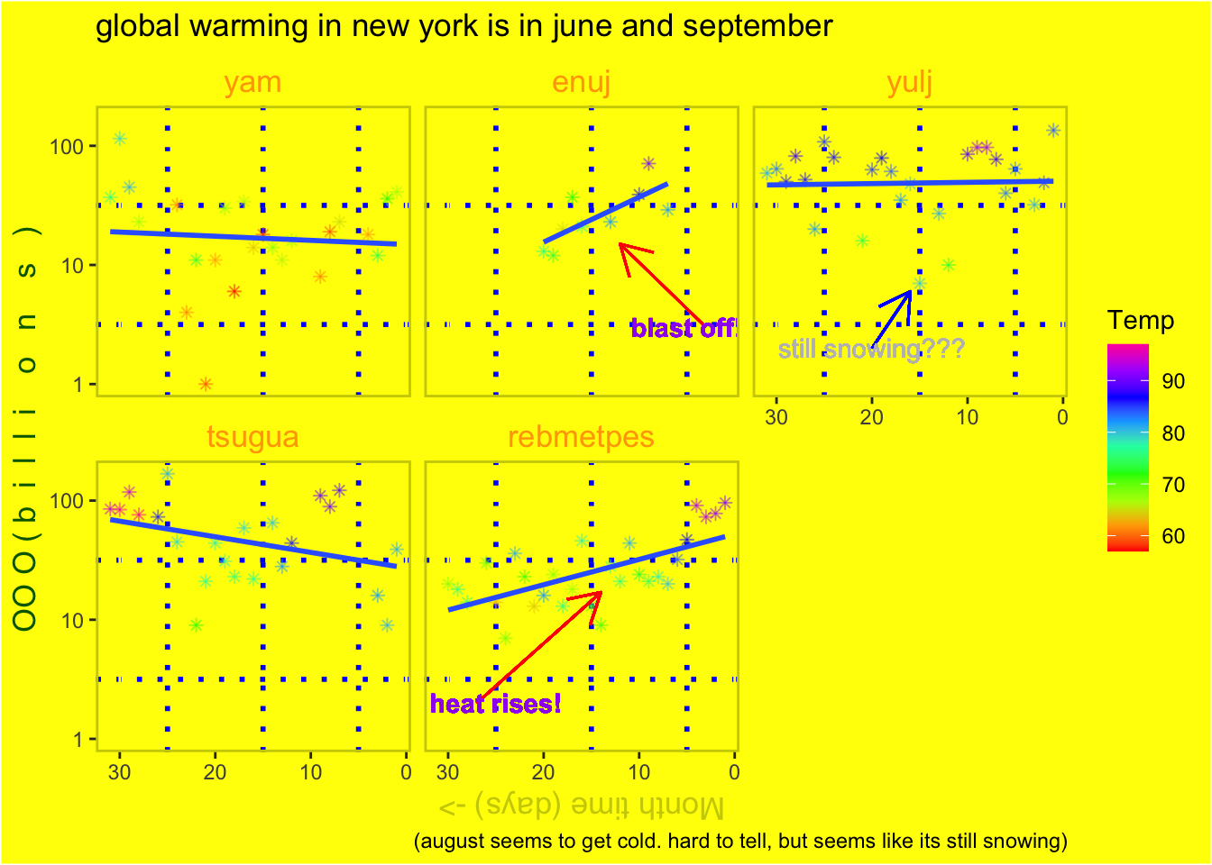
aqtib <- as_tibble(airquality) |>
  drop_na()

ggplot(
  aqtib,
  mapping = aes(
    x = Day,
    y = Ozone,
    color = Temp
  )
) +
  geom_point(shape = 8, alpha = 0.5) +
  scale_x_reverse() +
  scale_y_log10() +
  scale_color_gradientn(colours = rainbow(9)) +
  geom_smooth(method = lm, na.rm = FALSE, orientation = NA, se = FALSE) +
  facet_wrap(
    ~Month,
    labeller = labeller(
      Month = c(
        "5" = "yam",
        "6" = "enuj",
        "7" = "yulj",
        "8" = "tsugua",
        "9" = "rebmetpes"
      )
    )
  ) +
  labs(
    x = "Month time (days) ->",
    y = "OO O ( b  i  l  l  i    o   n    s   )",
    title = "global warming in new york is in june and september",
    caption = "(august seems to get cold. hard to tell, but seems like its still snowing)"
  ) +
  theme(
    plot.background = element_rect(fill = "yellow"),
    strip.background = element_blank(),
    strip.text = element_text(size = 13, color = "orange"),
    panel.border = element_rect(color = "yellow3", fill = NA, size = 1),
    panel.background = element_rect(fill = "yellow"),
    panel.grid.major = element_line(color = "yellow"),
    panel.grid.minor = element_line(
      color = "blue",
      linetype = "dotted",
      linewidth = 1
    ),
    axis.title.x = element_text(size = 13, color = "yellow3", angle = 180),
    axis.title.y = element_text(size = 13, color = "darkgreen"),
    legend.background = element_rect(fill = "yellow"),
  ) +
  geom_segment(
    data = subset(aqtib, Month == "6"),
    aes(x = 3, y = 3, xend = 12, yend = 15),
    arrow = arrow(length = unit(0.2, "inches")),
    color = "red"
  ) +
  geom_segment(
    data = subset(aqtib, Month == "7"),
    aes(x = 20, y = 2, xend = 16, yend = 6),
    arrow = arrow(length = unit(0.2, "inches")),
    color = "blue"
  ) +
  geom_segment(
    data = subset(aqtib, Month == "9"),
    aes(x = 27, y = 2, xend = 14, yend = 17),
    arrow = arrow(length = unit(0.2, "inches")),
    color = "red"
  ) +
  geom_text(
    data = subset(aqtib, Month == "6"),
    aes(x = 5, y = 3, label = "blast off!"),
    color = "purple",
    fontface = "bold"
  ) +
  geom_text(
    data = subset(aqtib, Month == "9"),
    aes(x = 25, y = 2, label = "heat rises!"),
    color = "purple",
    fontface = "bold"
  ) +
  geom_text(
    data = subset(aqtib, Month == "7"),
    aes(x = 20, y = 2, label = "still snowing???"),
    color = "grey"
  )

Plot 14

Code

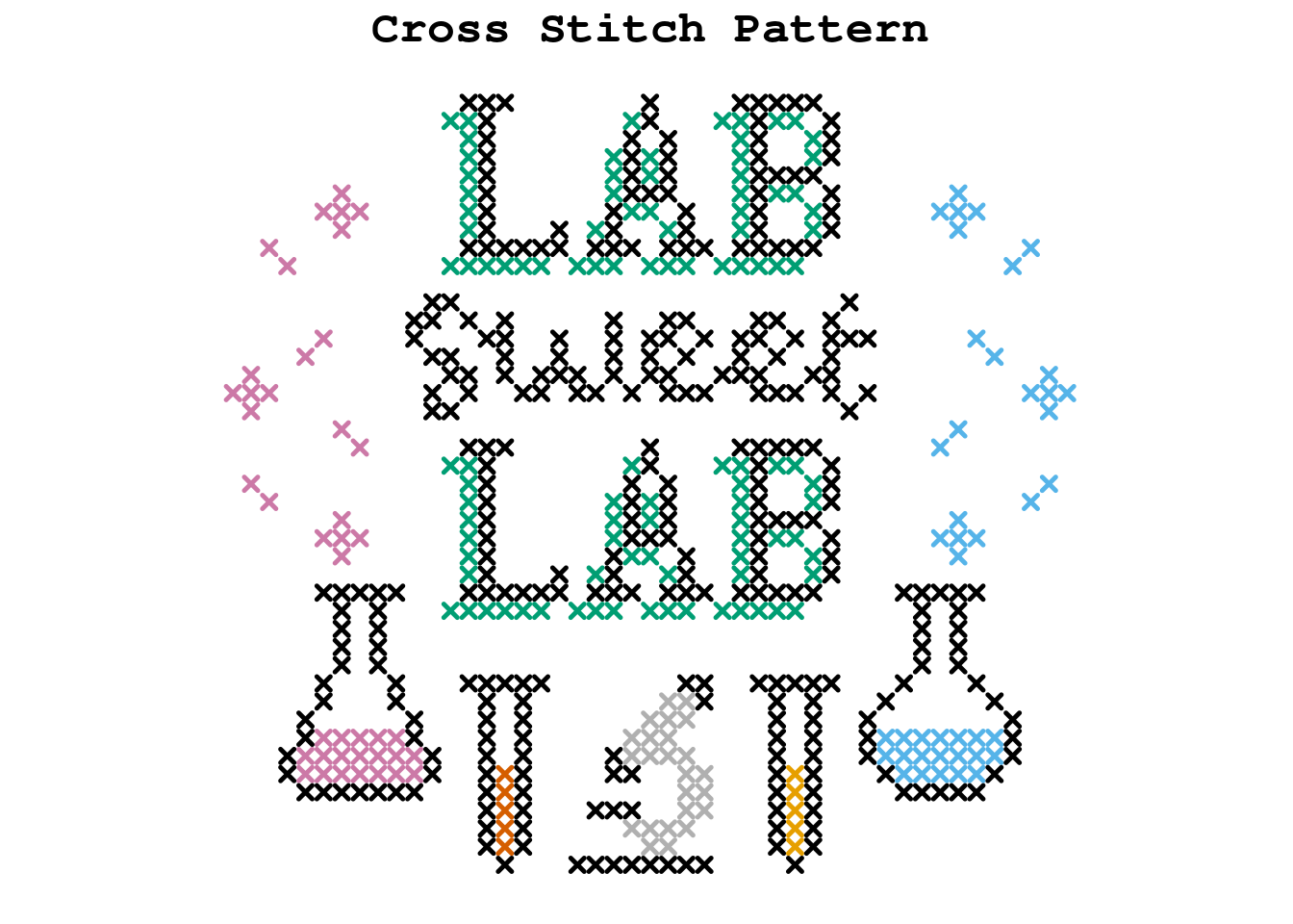
Pattern <- read_csv(here("Cross-Stitch-Pattern_250901.csv"))

Floss_colors <- c(
  "Black" = "#000000",
  "Cinnamon" = "#E69F00",
  "Fern Green" = "#009E73",
  "Raspberry - Light" = "#CC79A7",
  "Stone Grey - Dark" = "#B0B0B0",
  "Surf Blue - Light" = "#56B4E9",
  "Topaz - Light" = "#D55E00"
)

ggplot(
  Pattern,
  aes(x = x, y = y, color = color_name)
) +
  geom_point(
    shape = 4,
    size = 1.6,
    stroke = 1.3
  ) +
  scale_color_manual(values = Floss_colors) +
  coord_fixed(ratio = 1) +
  labs(
    x = NULL,
    y = NULL,
    title = "Cross Stitch Pattern"
  ) +
  theme(
    axis.text = element_blank(),
    axis.ticks = element_blank(),
    panel.background = element_blank(),
    legend.position = "none",
    plot.title = element_text(
      size = 18,
      face = "bold",
      family = "mono",
      hjust = 0.5
    )
  )

Plot 15

Code

library(tidyverse)
library(emo)
# library(emojifont)
library(here)
library(gganimate)
library(ragg)
data("WorldPhones")

set.seed(42)

worldphones_tidy <- WorldPhones %>%
  as.data.frame() %>%
  rownames_to_column(var = "year") %>%
  pivot_longer(
    cols = -year,
    names_to = "region",
    values_to = "phones"
  ) %>%
  mutate(
    emoji = case_when(
      region == "N.Amer" ~ emo::ji("eagle"),
      region == "Europe" ~ emo::ji("bear"),
      region == "Asia" ~ emo::ji("tiger"),
      region == "S.Amer" ~ emo::ji("monkey"),
      region == "Oceania" ~ emo::ji("penguin"),
      region == "Africa" ~ emo::ji("giraffe"),
      region == "Mid.Amer" ~ emo::ji("cow")
    )
  ) %>%
  select(
    year,
    emoji,
    region,
    phones
  )

ggplot(
  worldphones_tidy,
  aes(
    x = year,
    y = phones,
    color = region
  )
) +
  geom_text(
    aes(label = emoji),
    size = 4,
    show.legend = FALSE
  ) +
  labs(
    x = "BEST YEARS",
    y = "TOO MANY PHONES",
    title = "ANIMALS LOVE PHONES",
    caption = "eagles are addicted to phones"
  ) +
  scale_y_continuous(
    limits = c(0, 100000),
    breaks = seq(0, 100000, 10000),
    labels = scales::comma
  ) +
  scale_x_discrete(position = "top") +
  theme(
    axis.text.x = element_text(
      face = "bold",
      color = "#ffeda0",
      size = 13,
      angle = 179
    ),
    axis.text.y = element_text(
      face = "bold",
      color = "orange",
      size = 10,
      angle = 180
    ),
    plot.background = element_rect(fill = "pink"),
    plot.title = element_text(
      face = "bold.italic",
      color = "green",
      size = 18,
      angle = 183
    ),
    plot.caption = element_text(color = "white", size = 12),
    axis.title.x = element_text(size = 22, color = "dark blue", angle = 12),
    axis.title.y = element_text(color = "orange", angle = 181, size = 14),
    panel.background = element_rect(fill = "light blue")
  )
print(worldphones_tidy)

Plot 16

Code

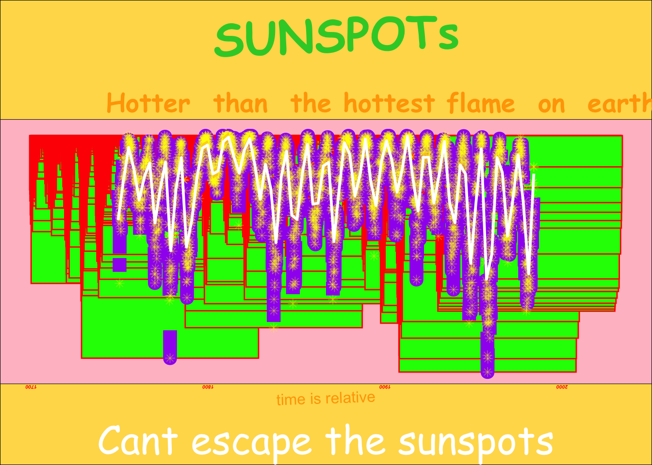
library(ggplot2)
library(tidyverse)
echo = TRUE
sun_tib <- tibble(
  year = as.numeric(time(sunspots)),
  sunspots = as.numeric(sunspots)
)

ggplot(
  sun_tib,
  aes(x = year, y = sunspots)
) +
  geom_bar(
    stat = "identity",
    fill = "green",
    color = "red",
    width = 100
  ) +
  geom_line(color = "purple", linewidth = 5, linetype = "dotdash") +
  geom_point(color = "yellow", size = 2, alpha = 0.3, shape = 8) +
  geom_smooth(
    method = "loess",
    span = .04,
    color = "white",
    fill = "orange",
    formula = y ~ x,
  ) +
  scale_y_reverse() +
  theme_void(base_size = 28) +
  theme(
    panel.background = element_rect(fill = "pink"),
    plot.background = element_rect(fill = "#FFDB58"),
    plot.title = element_text(
      color = "limegreen",
      face = "bold",
      hjust = 0.5,
      family = "Comic Sans MS",
      angle = 2,
      size = 35
    ),
    axis.text.x = element_text(
      face = "bold.italic",
      color = "red",
      size = 4,
      angle = 180
    ),
    axis.title.x = element_text(
      size = 12,
      color = "orange",
      angle = 2
    ),
    plot.subtitle = element_text(
      color = "orange",
      face = "bold",
      family = "Comic Sans MS",
      size = 20,
      hjust = ".4"
    ),
    plot.caption = element_text(
      color = "white",
      face = "italic",
      family = "Comic Sans MS",
      size = 30,
      hjust = ".5"
    )
  ) +
  labs(
    title = " SUNSPOTs",
    subtitle = "Hotter  than  the hottest flame  on  earth",
    caption = "Cant escape the sunspots",
    x = "time is relative",
    y = "spotty bois"
  )

Plot 17

Code

library(ggplot2)
library(dplyr)
library(purrr)
set.seed(1972)
library(gganimate)

letters_df <- data.frame(
  x = 1:4,
  y = 0,
  lab = c("A", "B", "B", "A"),
  col = c("#e91e63", "#ff8fc7", "#ff8fc7", "#e91e63") # pinks
)


shape_pool <- c(8, 3, 4, 18, 17)
n_sparkles <- 700
sparkles <- data.frame(
  x = runif(n_sparkles, 0.3, 4.7),
  y = runif(n_sparkles, -1.2, 1.2),
  size = runif(n_sparkles, 0.8, 3.0),
  alpha = runif(n_sparkles, 0.80, 1),
  col = sample(
    c("#f72585", "#ff5fa2", "#ff8fc7", "#ffd1e8", "#ffd166"),
    n_sparkles,
    TRUE
  ),
  shape = sample(shape_pool, n_sparkles, TRUE)
)

make_bursts <- function(n_bursts = 40, min_rays = 6, max_rays = 10) {
  centers <- data.frame(
    x0 = runif(n_bursts, 0.4, 4.6),
    y0 = runif(n_bursts, -1.1, 1.1)
  )
  bursts <- do.call(
    rbind,
    lapply(1:nrow(centers), function(i) {
      k <- sample(min_rays:max_rays, 1)
      th <- seq(0, 2 * pi, length.out = k + 1)[-(k + 1)]
      L <- runif(k, 0.05, 0.12)
      data.frame(
        x = centers$x0[i],
        y = centers$y0[i],
        xend = centers$x0[i] + L * cos(th),
        yend = centers$y0[i] + L * sin(th),
        alpha = runif(1, 0.08, 0.18),
        size = runif(1, 0.4, 0.9),
        col = sample(c("#f72585", "#ff8fc7", "#ffd1e8"), 1)
      )
    })
  )
  bursts
}
bursts <- make_bursts()

gg <- ggplot() +
  geom_segment(
    data = bursts,
    aes(
      x = x,
      y = y,
      xend = xend,
      yend = yend,
      alpha = alpha,
      size = size,
      color = col
    ),
    lineend = "round",
    show.legend = FALSE
  ) +
  geom_point(
    data = sparkles,
    aes(x, y, shape = shape, size = size, alpha = alpha, color = col),
    show.legend = FALSE
  ) +
  geom_text(
    data = letters_df,
    aes(x, y, label = lab, color = col),
    fontface = "bold",
    size = 30
  ) +
  scale_shape_identity() +
  scale_size_identity() +
  scale_alpha_identity() +
  scale_color_identity() +
  coord_cartesian(xlim = c(0.2, 4.8), ylim = c(-1.4, 1.4), expand = FALSE) +
  theme_void(base_size = 14) +
  theme(
    plot.background = element_rect(fill = "white", color = NA),
    panel.background = element_rect(fill = "white", color = NA),
    plot.margin = margin(30, 30, 30, 30)
  )

gg

Plot 18

Code

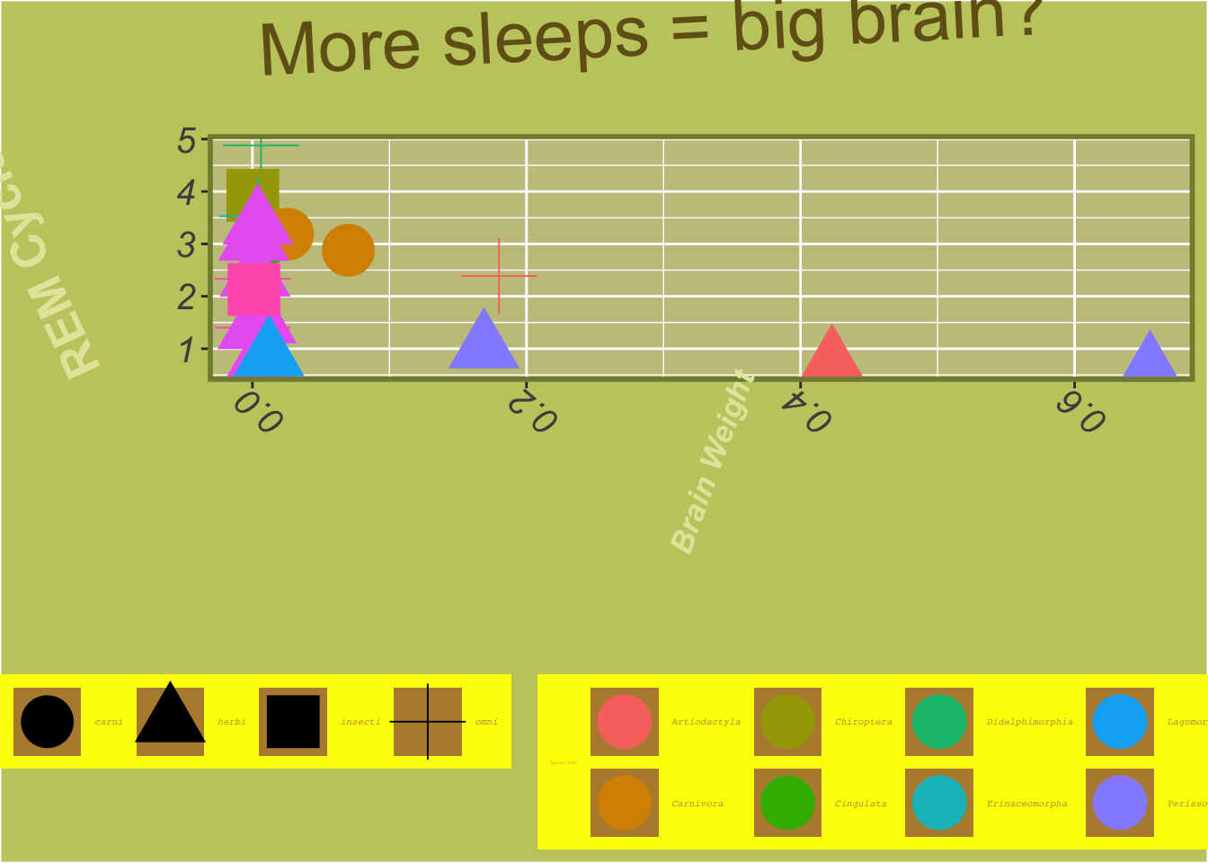
library(tidyverse)
library(ggplot2)

msleep_tbl <- drop_na(msleep)

ggplot(
  msleep_tbl,
  aes(
    x = brainwt,
    y = sleep_rem,
    color = order,
    shape = vore
  )
) +
  geom_jitter(size = 10) +
  theme(
    plot.background = element_rect(fill = "#c3cb6e"),
    plot.title = element_text(
      size = 30,
      hjust = 0.25,
      color = "#72601b",
      angle = 3
    ),
    plot.caption = element_text(size = 10, face = "italic", angle = 25),

    panel.background = element_rect(fill = '#c6c58b', size = 4),
    panel.border = element_rect(fill = 'NA', color = "#818c3c", size = 2),

    axis.title.x = element_text(
      face = "bold.italic",
      size = 13,
      color = "#e4e6a8",
      angle = 70
    ),
    axis.title.y = element_text(
      face = "bold",
      size = 20,
      color = "#e4e6a8",
      angle = 115
    ),
    axis.text = element_text(face = "italic", size = 15),
    axis.text.x.bottom = element_text(angle = 140),

    legend.background = element_rect(fill = "#fbff00"),
    legend.key = element_rect(fill = "#b78b3c"),
    #legend.direction = "vertical",
    legend.position = "bottom",
    #legend.justification = "left",
    legend.title = element_text(family = "serif", color = "#ef9e3a", size = 2),
    legend.text = element_text(
      family = "mono",
      face = "italic",
      color = "#c89c45",
      size = 4
    )
  ) +
  labs(
    title = "More sleeps = big brain?",
    x = "Brain Weight",
    y = "REM Cycles",
    col = "Species Order"
  )

Plot 19

Code

library(tidyverse)

set.seed(999)
n_layers <- 50
n_points <- 6

polys <- tibble()
for (i in 1:n_layers) {
  angle <- seq(0, 2 * pi, length.out = n_points + 1)[-1]
  radius <- runif(n_points, min = i * 0.5, max = i * 1.5)
  x <- radius * cos(angle) + rnorm(n_points, 0, 0.3)
  y <- radius * sin(angle) + rnorm(n_points, 0, 0.3)

  temp <- tibble(
    layer = i,
    x = x,
    y = y,
    fill = sample(c("#FF3C38", "#38FFDC", "#FFC738", "#8A38FF"), 1)
  )
  polys <- bind_rows(polys, temp)
}

n_rows <- nrow(polys)

ggplot(polys, aes(x = x, y = y, group = layer, fill = fill)) +
  geom_polygon(alpha = 0.5, color = "white", linewidth = 0.2) +
  geom_point(
    aes(
      x = x + rnorm(n_rows, 0, 0.1),
      y = y + rnorm(n_rows, 0, 0.1),
      color = fill
    ),
    size = 1,
    alpha = 0.7
  ) +
  scale_fill_identity() +
  scale_color_identity() +
  coord_fixed() +
  theme_void() +
  theme(
    plot.background = element_rect(fill = "#000000"),
    panel.background = element_rect(fill = "#000000")
  )

Plot 20

Code

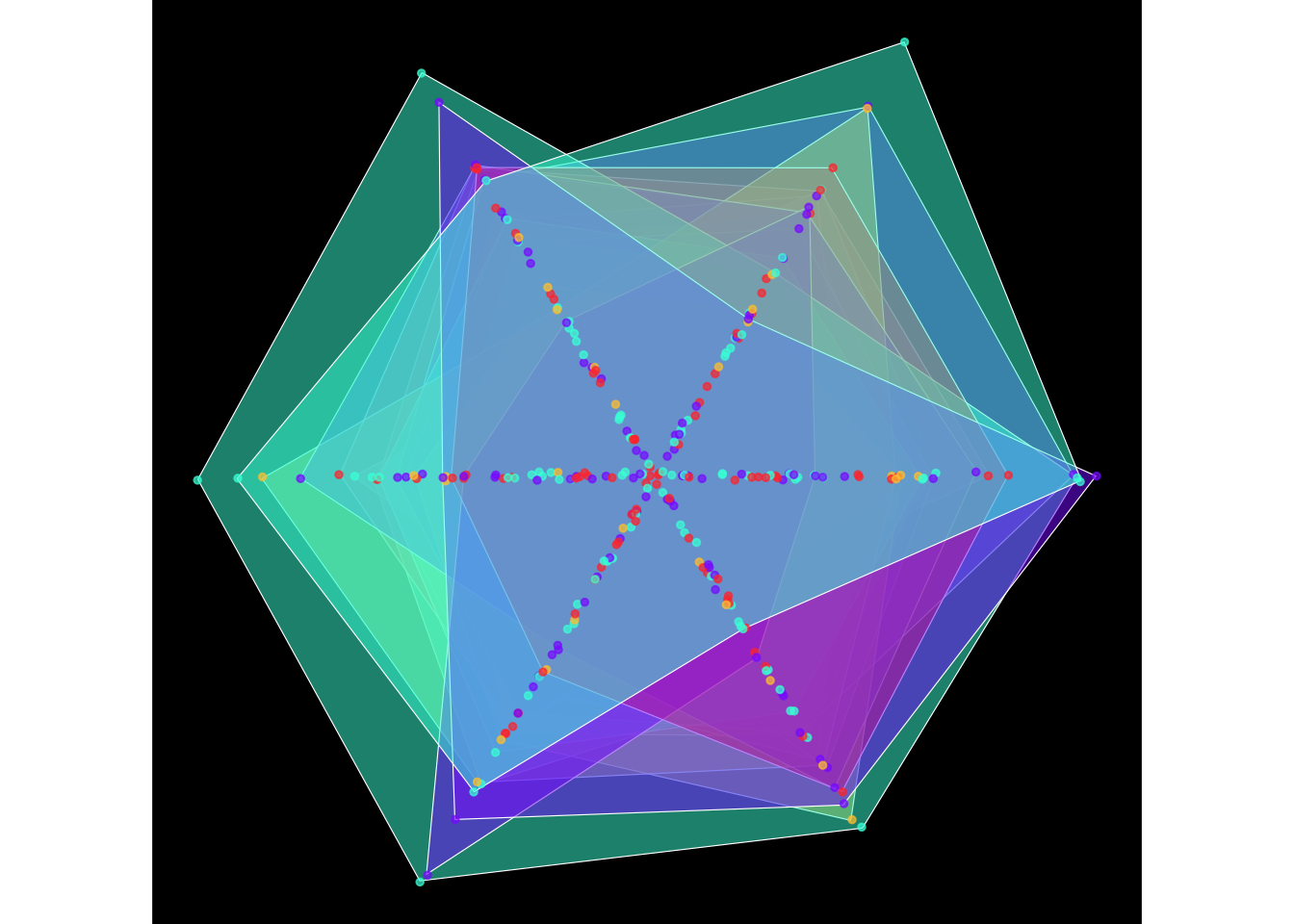
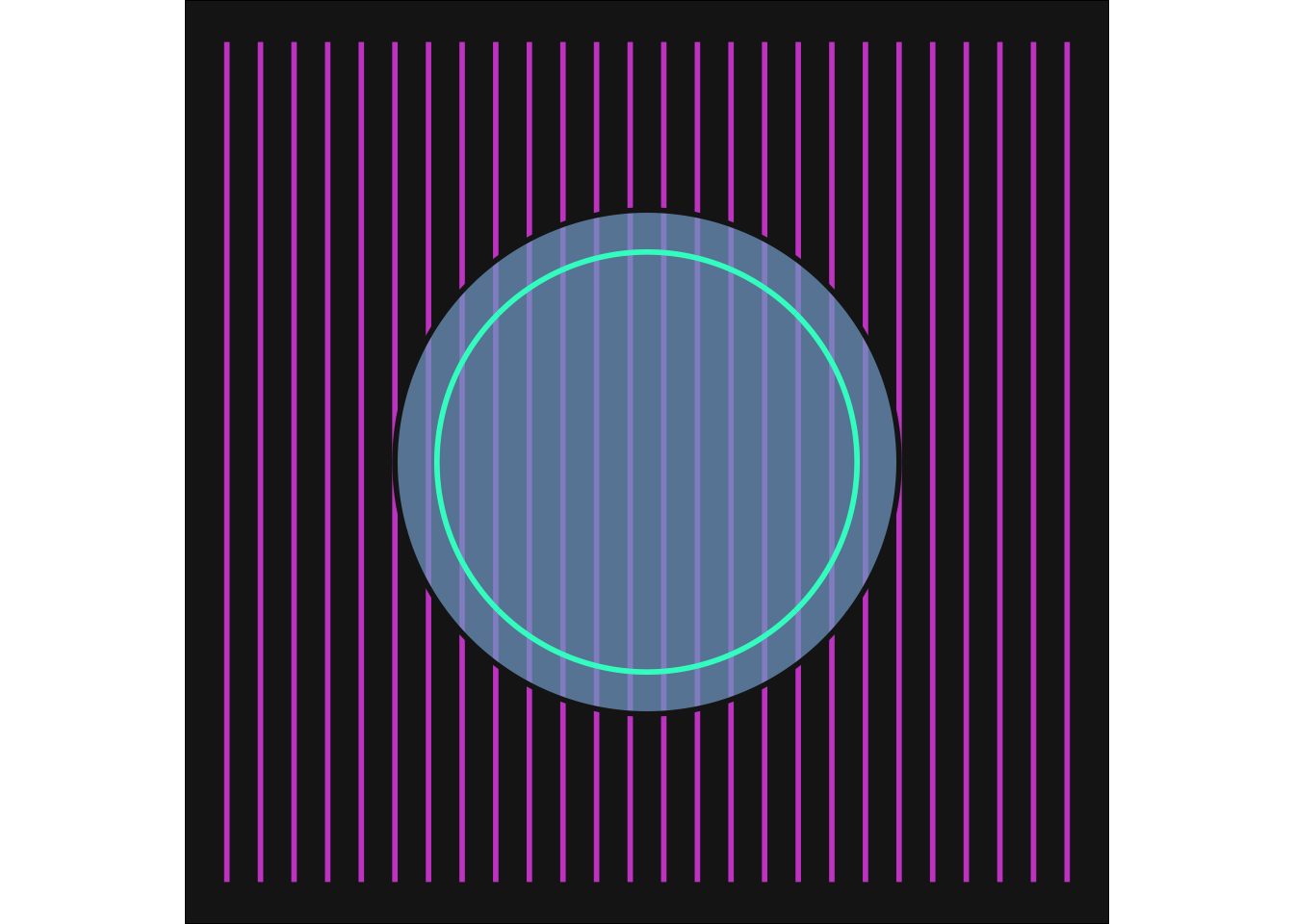
library(ggplot2)
library(ggforce)
library(RColorBrewer)
library(dplyr)

hori_lines <- tibble(
  x = seq(1, -1, by = -.08),
  xend = seq(1, -1, by = -.08),
  y = -1,
  yend = 1
)

inner_circle <- tibble(
  x = 0,
  y = 0,
  radius = 0.6
)

arc <- tibble(
  x = 0,
  y = 0,
  r = .5,
  start = seq(0, 2 * pi, length.out = 9)[-9],
  end = seq(0, 2 * pi, length.out = 9)[-1],
  type = c("A", "B", "B", "A", "A", "B", "B", "A")
)

neon_rain_palette <- c("#32faca", "#58d0cb", "#7fa5cb", "#a57bcc", "#cc51cd")

p <- ggplot() +

  geom_segment(
    data = hori_lines,
    aes(x = x, xend = xend, y = y, yend = yend, color = "lines"),
    size = 1
  ) +

  geom_circle(
    data = inner_circle,
    aes(x0 = x, y0 = y, r = radius, fill = "circle_fill"),
    size = 1,
    alpha = 0.75,
    color = "#1A1A1A" # Dark border to contrast with the neon colors
  ) +

  geom_arc(
    data = arc,
    aes(
      x0 = x,
      y0 = y,
      r = r,
      start = start,
      end = end,
      color = "arc_lines",
      type = type
    ),
    size = 1
  ) +

  scale_color_manual(
    values = c(
      "lines" = neon_rain_palette[5], # A bright purple for the lines
      "arc_lines" = neon_rain_palette[1] # A bright teal for the arc
    )
  ) +

  scale_fill_manual(
    values = c(
      "circle_fill" = neon_rain_palette[3] # A muted blue for the circle fill
    )
  ) +

  coord_fixed() +
  theme_void() +
  theme(
    legend.position = "none",
    plot.background = element_rect(fill = "#1A1A1A")
  )

print(p)