DNA Block - Problem Set 18

Problem Set

Total points: 20. First problem is worth 7 points, second problem is worth 13 points.

Load libraries

Start by loading libraries you need analysis in the code chunk below.

library(tidyverse)
library(here)
library(cowplot)
library(valr)

Load the data from the MNase-seq experiment.

mnase_tbl <- read_bed(
  here("data/block-dna/yeast_mnase_chrII.bed.gz")
)

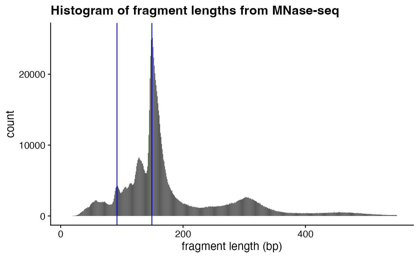
In class we learned that MNase digestion yields nucleosomal “footprints” of ~150 bp in size. I’ve added blue vertical lines to emphasize positions of the major peak (intact nucleosomes) as well as smaller “sub-nucleosomal” peak.

We can calculate the counts for the histogram above and more precisely determine the maximum signal using which.max() to identify the index of the maximum value in a vector (not the value itself!):

frag_hist <-
  mnase_tbl |>
  mutate(frag_len = end - start) |>
  count(frag_len)

# `which.max` takes a vector and gives us the index of the maximum value
max_idx <- which.max(frag_hist$n)

# now we can use index to find the abundant fragment size.
# we'll use `ncp_max` later in question 2.
ncp_max <- frag_hist$frag_len[max_idx]

So this tells us that that the most abundant fragment size in the library is ??? bp.

Question 1 – 7 points

Let’s take a closer look at the some of the smaller fragments in the MNase experiment. In particular, let’s zoom in on the populations of fragments that are smaller than 1 nucleosome in size, the peak between 85 and 95 bp (the left-most blue vertical line).

1. Use the above strategy to precisely determine the peak of this smaller size range. How big are those fragments? These are called “sub-nucleosomal” fragments.

# store the maximum value in `subnuc_max`. we'll use it later in question 2.

The maximum sub-nucleosomal fragments size is ??? bp.

2. Do this one more time, and identify the position of maximum signal in the disome peak (i.e., the fragments protected by two nucleosomes).

3. Recreate the histogram using ggplot2 (using relevant code from class 17) and add the blue vertical lines at the peak positions you calculated, including the position of the disomes above.

Question 2 – 13 points

Next we’re going to look at where these sub-sucleosomes are with respect to intact nucleosomes.

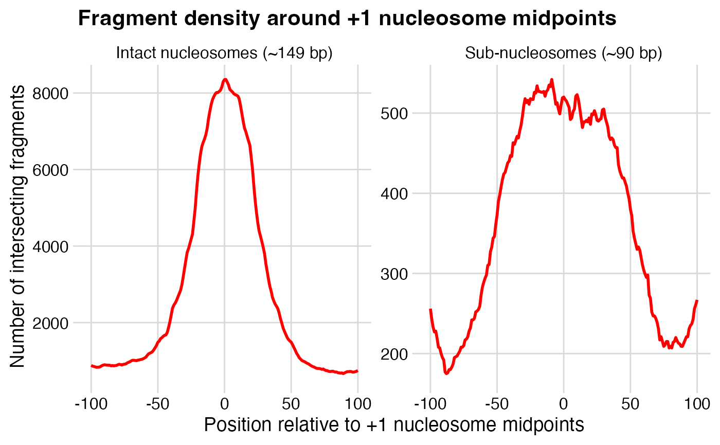
Our strategy will be to compare the density of sub-nucleosomes relative to the mid-points of previously mapped nucleosomes. Specifically, our reference point will be the midpoints of the +1 nucleosomes.

So you’ll make a metaplot, but instead of using transcription start sites as the reference point, we’ll use the midpoints of the +1 nucleosome, and instead of MNase-seq signal density, you’ll count up the number of individual reads that intersect with windows around those midpoints.

1. First, load the relevant data. We’ll re-use the yeast_mnase_chrII.bed.gz data you loaded above, plus you’ll need to load two other files:

   • a “genome” file, sacCer3.chrom.sizes
   • a BED file, yeast_p1_chrII.bed.gz which contains the mid-points of the +1 nucleosomes on chromosome 22. Recall that the +1 nucleosome is the nucleosome downstream of the transcription start site.

genome <- read_???(here("data/block-dna/sacCer3.chrom.sizes"))
p1_tbl <- read_???(here("data/block-dna/yeast_p1_chrII.bed.gz"))

2. Next, we need the mid-points of nucleosomes for comparison. The following function needs fixing. The midpoint is the coordinate halfway between the start and end of a given interval.

   You’re going to provide the mnase_tbl defined in question 1 to this function, which then:

   • calculates fragment lengths

   • filters them based on min_len and max_len

   • calculates the midpoints for each interval

   The output is a new tibble with columns `chrom`, `start`, and `end`.

calc_mids <- function(tbl, min_len, max_len) {
  tbl |>
    mutate(
      frag_len = ___ - ___
    ) |>
    filter(
      frag_len >= ___ & frag_len <= ___
    ) |>
    mutate(
      # calculate the half-size interval using `end` and `start,
      # then add that value to `start`
      midpoint = ___
    ) |>
    select(chrom, midpoint) |>
    rename(start = midpoint) |>
    mutate(end = start + 1)
}

3. Next, use that function to calculate midpoints, and expand these midpoints by 20 bp in each direction with bed_slop().

ncp_mids_tbl <-
  # first calculate midpoints for nucleosome fragments within 3 bp length `ncp_max`
  calc_mids(mnase_tbl, ___ - 3, ___ + 3) |>
  # expand those windows to get a larter window for intersection
  bed_slop(genome, both = 20)

# now, do the same for nucleosome fragments of length `subnuc_max`
subnuc_mids_tbl <-
  calc_mids(mnase_tbl, ___ - 3, ___ + 3) |>
  bed_slop(genome, both = 20)

4. Next, we need to make the reference points for a metaplot. We’ll look 100 bp up- and downstream of the +1 nucleosome positions, and make windows that are 1 bp in size.

p1_win_tbl <-
  bed_???(
    p1_tbl,
    genome,
    both = 100
  ) |>
  bed_???(win_size = 1)

5. Almost there! Now you just need to identify the number of short and long nuclesome fragments (based on their midpoints) that intersect with the +1 nucleosomes you defined above.

   Use bed_intersect() to identify fragments that overlap, and then just count the number of fragments per .win_id (don’t forget the suffix). Note you will do this separately for the short and long fragments.

ncp_mids_summary_tbl <-
  bed_intersect(
    p1_win_tbl,
    ncp_mids_tbl
  ) |>
  dplyr::count(___) |>
  mutate(type = "Intact nucleosomes (~149 bp)")

subnuc_mids_summary_tbl <-
  bed_intersect(
    p1_win_tbl,
    subnuc_mids_tbl
  ) |>
  dplyr::count(___) |>
  mutate(type = "Sub-nucleosomes (~90 bp)")

6. The following joins the tables you made together, and makes the x-axis more informative, by converting to relative genomic position rather than window ID.

win_ids <- seq(-100, 100, 1)

all_tbl <- bind_rows(
  ncp_mids_summary_tbl,
  subnuc_mids_summary_tbl
) |>
  mutate(win_ids = win_ids, .by = "type")

7. Finally, we plot the data with position on the x-axis, and count on the y-axis.

ggplot(
  all_tbl,
  aes(win_ids, n)
) +
  geom_???(color = "red") +
  facet_wrap(
    ~ type,
    scales = "free_y"
  ) +
  theme_minimal_grid() +
  labs(
    x = "Position relative to +1 nucleosome midpoints",
    y = "Number of intersecting fragments",
    title = "Fragment density around +1 nucleosome midpoints"
  )

Output

Your plot should look like this.

Plot output of step 7

Interpretation

How do you interpret these plots?

Rationalize the pattern for intact nucleosomes. What pattern did you expect to see?

Answer.

Rationalize the pattern for sub-nucleosomes. How would you describe the positions of sub-nucleosomal fragments, relative to the +1 nucleosome midpoints? What might this mean with respect to gene transcription?

Answer.

What do the differences between signal magnitudes (reflected by the y-axis) mean?

Answer.

Submit

Be sure to click the “Render” button to render the HTML output. Then paste the URL of this Posit Cloud project into the problem set on Canvas.