RNAseq DE

Matthew Taliaferro

RNA Bioscience Initiative | CU Anschutz

2026-09-25

Overview

Last time we took RNAseq data from an in vitro differentiation timecourse from mouse ESCs to glutaminergic neurons (Hubbard et al, F1000 Research (2013)). We took in transcript-level quantifications produced by salmon and collapsed them to gene-level quantifications using tximport. We then inspected the quality of the data by relating distances between samples using two methods: hierarchical clustering and principal components analysis. We found that the data was of high quality, as evidenced by the fact that replicates from a given timepoint were highly similar to other replicates for the same timepoint, and the distances between samples made sense with what we know about how the experiment was conducted.

Today, we are going to pretend that this isn’t a timecourse. For the sake of simplicity, we are going to imagine that we have only two conditions: DIV0 and DIV7. We will use DESeq2 to identify genes that are differentially expressed between these two timepoints. We will then plot changes in expression for both individual genes and groups of genes that we already know going in might be interesting to look at. Finally, we will look at some features of transcripts and genes that are differentially expressed between these two timepoints.

Prepare t2g

The first thing we need to do is read in the data again and move from transcript-level expression values to gene-level expression values with tximport. To save time and space, read in a pre-computed t2g table. If you need to refresh yourself on how t2g was created, refer to the slides or exercises from the previous class.

t2g <- read_tsv(here("data", "block-rna", "t2g.tsv.gz"))

Rows: 149547 Columns: 3
── Column specification ────────────────────────────────────
Delimiter: "\t"
chr (3): ensembl_transcript_id, ensembl_gene_id, externa...

ℹ Use `spec()` to retrieve the full column specification for this data.
ℹ Specify the column types or set `show_col_types = FALSE` to quiet this message.

# maps systematic to common gene names
gene_name_map <- t2g |>
  dplyr::select(-ensembl_transcript_id) |>
  unique()

Prepare metadata and import

Now we can read in the transcript-level data and collapse to gene-level data with tximport

metadata <- tibble(
  salmon_dirs = fs::dir_ls(
    here("data/block-rna/differentiation_salmonouts"),
    recurse = TRUE,
    glob = "*quant.sf"
  )
) |>
  mutate(
    sample_id = fs::path_file(fs::path_dir(salmon_dirs))
  ) |>
  filter(str_starts(sample_id, "DIV")) |>
  separate_wider_delim(
    col = sample_id,
    delim = ".",
    names = c("timepoint", "rep"),
    too_few = "align_start",
    cols_remove = FALSE
  ) |>
  mutate(rep = str_remove(rep, "Rep")) |>
  column_to_rownames("sample_id")

# Add the sample_id column back from rownames
metadata$sample_id <- rownames(metadata)

metadata <- metadata |>
  filter(
    timepoint %in% c("DIV0", "DIV7")
  )

salmdir <- metadata$salmon_dirs
names(salmdir) <- metadata$sample_id

txi <- tximport(
  files = salmdir,
  type = "salmon",
  tx2gene = t2g,
  dropInfReps = TRUE,
  countsFromAbundance = "lengthScaledTPM"
)

reading in files with read_tsv

1 2 3 4 5 6 7 
transcripts missing from tx2gene: 3733
summarizing abundance
summarizing counts
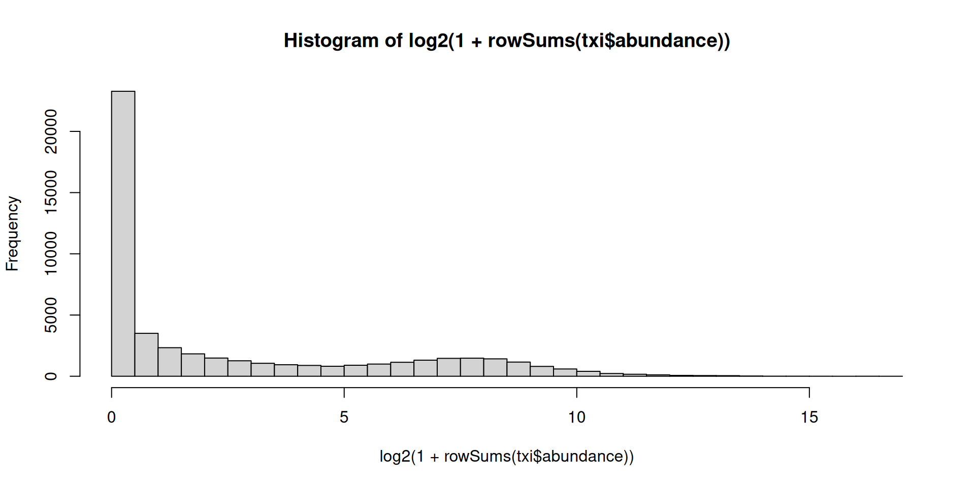
summarizing length

Filter lowly expressed genes

# examine distribution of TPMs
hist(log2(1 + rowSums(txi$abundance)), breaks = 40)

# decide a cutoff
keepG <- txi$abundance[log2(1 + rowSums(txi$abundance)) > 4.5, ] |>
  rownames()

Create DESeq object

There are essentially two steps to using DESeq2. The first involves creating a DESeqDataSet from your data. Luckily, if you have a tximport object, which we do in the form of txi, then this becomes easy.

ddsTxi <- DESeqDataSetFromTximport(
  txi,
  colData = metadata,
  design = ~timepoint
)

Warning in DESeqDataSet(se, design = design, ignoreRank):
some variables in design formula are characters, converting
to factors

using just counts from tximport

# keep genes with sufficient expession
ddsTxi <- ddsTxi[keepG, ]

Design formula

You can see that DESeqDataSetFromTximport wants three things. The first is our tximport object. The second is the dataframe we made that relates samples and conditions (or in this case timepoints). The last is something called a design formula. A design formula contains all of the variables that will go into DESeq2’s model. The formula starts with a tilde and then has variables separated by a plus sign think lm(). It is common practice, and in fact basically required with DESeq2, to put the variable of interest last. In our case, that’s trivial because we only have one: timepoint. So our design formula is very simple:

design = ~ timepoint

Your design formula should ideally include all of the sources of variation in your data. For example, let’s say that here we thought there was a batch effect with the replicates. Maybe all of the Rep1 samples were prepped and sequenced on a different day than the Rep2 samples and so on. We could potentially account for this in DESeq2’s model with the following forumula:

design = ~ rep + timepoint

Here, timepoint is still the variable of interest, but we are controlling for differences that arise due to differences in replicates.

Run DESeq2

We can see here that DESeq2 is taking the counts produced by tximport for gene quantifications. There are 52346 genes (rows) here and 7 samples (columns). Now using this ddsTxi object, we can run DESeq2.

# create DESeq object
dds <- DESeq(ddsTxi)

estimating size factors

estimating dispersions

gene-wise dispersion estimates

mean-dispersion relationship

final dispersion estimates

fitting model and testing

There are many useful things in this dds object. Take a look at the vignette for a full explanation. Including info on many more tests and analyses that can be done with DESeq2.

The results can be accessed using the results() function. We will use the contrast argument here. DESeq2 reports changes in RNA abundance between two samples as a log2FoldChange. But, it’s often not clear what the numerator and denominator of that fold change ratio…it could be either DIV7/DIV0 or DIV0/DIV7.

The lexographically first condition will be the numerator. I find it easier to explicitly specify what the numerator and denominator of this ratio are using the contrast argument. The contrast argument can be used to implement more complicated design formula. Remember our design formula that accounted for potential differences due to Replicate batch effects:

~ replicate + timepoint

DESeq2 will account for differences between replicates here to find differences between timepoints.

Contrasts to get results

# For contrast, we give three strings: the factor we are interested in, the numerator, and the denominator
results(dds, contrast = c("timepoint", "DIV7", "DIV0"))

log2 fold change (MLE): timepoint DIV7 vs DIV0 
Wald test p-value: timepoint DIV7 vs DIV0 
DataFrame with 13211 rows and 6 columns
                     baseMean log2FoldChange     lfcSE
                    <numeric>      <numeric> <numeric>
ENSMUSG00000000001   5616.933      -0.951431 0.0532718
ENSMUSG00000000028    723.248      -2.551794 0.1073992
ENSMUSG00000000031   3651.758       4.121821 0.2929827
ENSMUSG00000000037    244.281      -1.273199 0.2045431
ENSMUSG00000000056   2391.002       0.788852 0.1469530
...                       ...            ...       ...
ENSMUSG00000121504  662.57656      -0.917131 0.0801445
ENSMUSG00000121583 1650.63790       0.367053 0.0494672
ENSMUSG00000121584  590.50603       1.531478 0.0864644
ENSMUSG00002076020    2.70252       1.186067 1.1740531
ENSMUSG00002076083 1281.79977       0.892433 0.0599871
                        stat       pvalue         padj
                   <numeric>    <numeric>    <numeric>
ENSMUSG00000000001 -17.85994  2.41879e-71  1.14360e-70
ENSMUSG00000000028 -23.75990 8.68157e-125 7.28612e-124
ENSMUSG00000000031  14.06848  5.93327e-45  1.96339e-44
ENSMUSG00000000037  -6.22460  4.82789e-10  7.93733e-10
ENSMUSG00000000056   5.36806  7.95901e-08  1.21970e-07
...                      ...          ...          ...
ENSMUSG00000121504 -11.44348  2.53507e-30  6.58700e-30
ENSMUSG00000121583   7.42013  1.17002e-13  2.12834e-13
ENSMUSG00000121584  17.71224  3.37385e-70  1.57542e-69
ENSMUSG00002076020   1.01023  3.12384e-01  3.39441e-01
ENSMUSG00002076083  14.87710  4.64181e-50  1.64569e-49

The columns we are most interested in are log2FoldChange and padj.

log2FoldChange is self-explanatory. padj is the Benjamini-Hochberg corrected pvalue for a test asking if the expression of this gene is different between the two conditions.

Cleanup results

Let’s do a little work on this data frame to make it slightly cleaner and more informative.

diff <-
  results(
    dds,
    contrast = c("timepoint", "DIV7", "DIV0")
  ) |>
  # Change this into a dataframe
  as.data.frame() |>
  # Move ensembl gene IDs into their own column
  rownames_to_column(var = "ensembl_gene_id") |>
  as_tibble() |>
  # drop unused columns
  dplyr::select(-c(baseMean, lfcSE, stat, pvalue)) |>
  # Merge this with a table relating ensembl_gene_id with gene short names
  inner_join(gene_name_map) |>
  # Rename external_gene_name column
  dplyr::rename(gene = external_gene_name)

Joining with `by = join_by(ensembl_gene_id)`

How many are significant

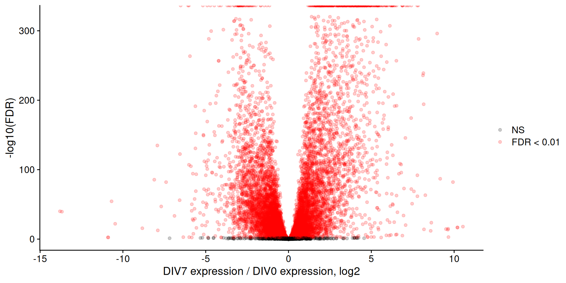
OK now we have a table of gene expression results. How many genes are significantly up/down regulated between these two timepoints? We will use 0.01 as an FDR (p.adj) cutoff.

# number of upregulated genes
nrow(filter(diff, padj < 0.01 & log2FoldChange > 0))

[1] 5301

# number of downregulated genes
nrow(filter(diff, padj < 0.01 & log2FoldChange < 0))

[1] 5333

Volcano plot of differential expression results

Let’s make a volcano plot of these results.

# meets the FDR cutoff
diff_sig <-
  mutate(
    diff,
    sig = case_when(
      padj < 0.01 ~ "yes",
      .default = "no"
    )
  ) |>
  # if a gene did not meet expression cutoffs that DESeq2 automatically does, it gets a pvalue of NA
  drop_na()

ggplot(
  diff_sig,
  aes(
    x = log2FoldChange,
    y = -log10(padj),
    color = sig
  )
) +
  geom_point(alpha = 0.2) +
  labs(
    x = "DIV7 expression / DIV0 expression, log2",
    y = "-log10(FDR)"
  ) +
  scale_color_manual(
    values = c("black", "red"),
    labels = c("NS", "FDR < 0.01"),
    name = ""
  ) +
  theme_cowplot()

Volcano plot of differential expression results

Change the LFC threshold

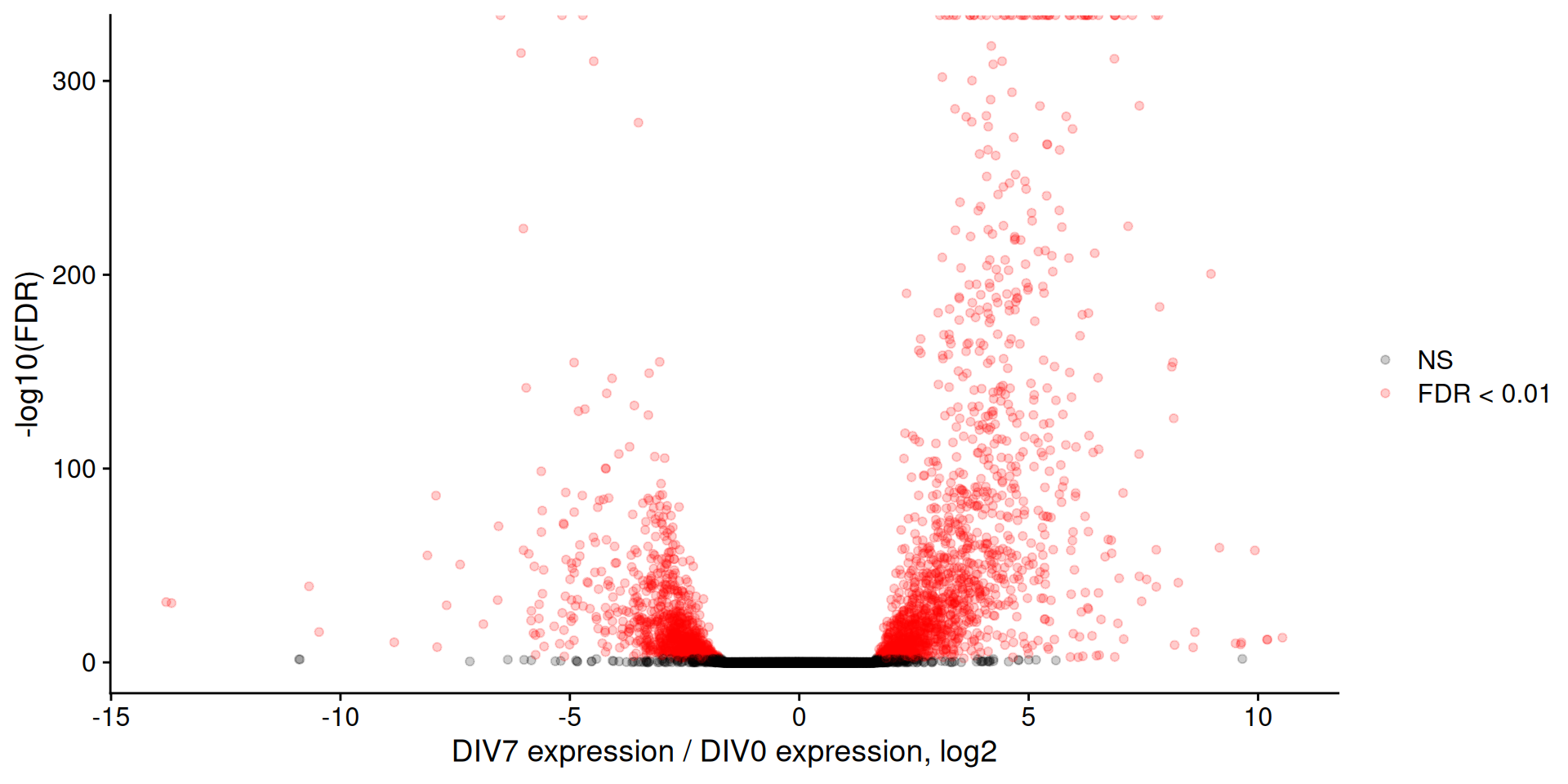
In addition to an FDR cutoff, let’s also apply a log2FoldChange cutoff. This will of course be more conservative, but will probably give you a more confident set of genes.

# Is the expression of the gene at least 3-fold different?
diff_lfc <-
  results(
    dds,
    contrast = c("timepoint", "DIV7", "DIV0"),
    lfcThreshold = log(3, 2)
  ) |>
  # Change this into a dataframe
  as.data.frame() |>
  # Move ensembl gene IDs into their own column
  rownames_to_column(var = "ensembl_gene_id") |>
  as_tibble() |>
  # drop unused columns
  select(-c(baseMean, lfcSE, stat, pvalue)) |>
  # Merge this with a table relating ensembl_gene_id with gene short names
  inner_join(gene_name_map) |>
  # Rename external_gene_name column
  dplyr::rename(gene = external_gene_name)

Joining with `by = join_by(ensembl_gene_id)`

# number of upregulated genes
nrow(
  filter(
    diff_lfc,
    padj < 0.01 & log2FoldChange > 0
  )
)

[1] 1511

# number of downregulated genes
nrow(
  filter(
    diff_lfc,
    padj < 0.01 & log2FoldChange < 0
  )
)

[1] 990

Change the LFC threshold

diff_lfc_sig <-
  mutate(
    diff_lfc,
    sig = case_when(
      padj < 0.01 ~ "yes",
      .default = "no"
    )
  ) |>
  drop_na()


# look at some specific genes

diff_lfc_sig |>
  filter(
    gene %in%
      c("Bdnf", "Dlg4", "Klf4", "Sox2")
  ) |>
  gt()

ensembl_gene_id	log2FoldChange	padj	gene	sig
ENSMUSG00000003032	-2.344594	3.984536e-09	Klf4	yes
ENSMUSG00000020886	3.338654	1.391036e-45	Dlg4	yes
ENSMUSG00000048482	1.709765	4.929354e-01	Bdnf	no
ENSMUSG00000074637	-2.169991	4.331519e-13	Sox2	yes

Filtered Volcano

ggplot(
  diff_lfc_sig,
  aes(
    x = log2FoldChange,
    y = -log10(padj),
    color = sig
  )
) +
  geom_point(alpha = 0.2) +
  labs(
    x = "DIV7 expression / DIV0 expression, log2",
    y = "-log10(FDR)"
  ) +
  scale_color_manual(
    values = c("black", "red"),
    labels = c("NS", "FDR < 0.01"),
    name = ""
  ) +
  theme_cowplot()

Filtered Volcano

Plotting the expression of single genes

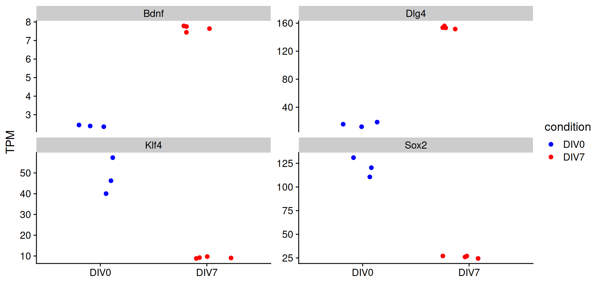
Sometimes we will have particular marker genes that we might want to highlight to give confidence that the experiment worked as expected. We can plot the expression of these genes in each replicate. Let’s plot the expression of two pluripotency genes (which we expect to decrease) and two neuronal genes (which we expect to increase).

So what is the value that we would plot? We could use the ‘normalized counts’ value provided by DESeq2. However, remember there is not length calculation so it is difficult to compare accross genes.

A more interpretable value to plot might be TPM, since TPM is length-normalized. Let’s say a gene was expressed at 500 TPM. Right off the bat, I know generally what kind of expression that reflects (pretty high).

Get TPMs

Let’s plot the expression of Klf4, Sox2, Bdnf, and Dlg4 in our samples.

tpms <- txi$abundance |>
  as.data.frame() |>
  rownames_to_column(var = "ensembl_gene_id") |>
  as_tibble() |>
  inner_join(gene_name_map) |>
  dplyr::rename(gene = external_gene_name) |>
  # Filter for genes we are interested in
  filter(gene %in% c("Klf4", "Sox2", "Bdnf", "Dlg4")) |>
  pivot_longer(-c(ensembl_gene_id, gene)) |>
  separate_wider_delim(
    col = name,
    delim = ".",
    names = c("condition", "rep")
  )

Get TPMs

Joining with `by = join_by(ensembl_gene_id)`

gt(tpms)

ensembl_gene_id	gene	condition	rep	value
ENSMUSG00000003032	Klf4	DIV0	Rep1	40.022629
ENSMUSG00000003032	Klf4	DIV0	Rep2	46.241797
ENSMUSG00000003032	Klf4	DIV0	Rep3	57.374566
ENSMUSG00000003032	Klf4	DIV7	Rep1	9.063035
ENSMUSG00000003032	Klf4	DIV7	Rep2	9.208364
ENSMUSG00000003032	Klf4	DIV7	Rep3	9.715119
ENSMUSG00000003032	Klf4	DIV7	Rep4	8.817037
ENSMUSG00000020886	Dlg4	DIV0	Rep1	18.752921
ENSMUSG00000020886	Dlg4	DIV0	Rep2	15.749749
ENSMUSG00000020886	Dlg4	DIV0	Rep3	12.212636
ENSMUSG00000020886	Dlg4	DIV7	Rep1	151.558403
ENSMUSG00000020886	Dlg4	DIV7	Rep2	156.043098
ENSMUSG00000020886	Dlg4	DIV7	Rep3	153.269475
ENSMUSG00000020886	Dlg4	DIV7	Rep4	153.538436
ENSMUSG00000048482	Bdnf	DIV0	Rep1	2.456452
ENSMUSG00000048482	Bdnf	DIV0	Rep2	2.401157
ENSMUSG00000048482	Bdnf	DIV0	Rep3	2.351342
ENSMUSG00000048482	Bdnf	DIV7	Rep1	7.799981
ENSMUSG00000048482	Bdnf	DIV7	Rep2	7.762255
ENSMUSG00000048482	Bdnf	DIV7	Rep3	7.638515
ENSMUSG00000048482	Bdnf	DIV7	Rep4	7.433529
ENSMUSG00000074637	Sox2	DIV0	Rep1	131.032132
ENSMUSG00000074637	Sox2	DIV0	Rep2	120.433905
ENSMUSG00000074637	Sox2	DIV0	Rep3	110.664468
ENSMUSG00000074637	Sox2	DIV7	Rep1	24.484942
ENSMUSG00000074637	Sox2	DIV7	Rep2	26.080394
ENSMUSG00000074637	Sox2	DIV7	Rep3	27.106054
ENSMUSG00000074637	Sox2	DIV7	Rep4	26.995461

Now plot

ggplot(
  tpms,
  aes(
    x = condition,
    y = value,
    color = condition
  )
) +
  geom_jitter(size = 2, width = .25) +
  labs(
    x = "",
    y = "TPM"
  ) +
  theme_cowplot() +
  scale_color_manual(values = c("blue", "red")) +
  facet_wrap(~gene, scales = "free_y")

How about pathways?

Say that instead of plotting individual genes we wanted to ask whether a whole class of genes are going up or down. We can do that by retrieving all genes that belong to a particular gene ontology term.

There are three classes of genes we will look at here:

• Maintenance of pluripotency (GO:0019827)
• Positive regulation of the cell cycle (GO:0045787)
• Neuronal differentitaion (GO:0030182)

Retrieve pathway information

We can use ensembl to get all genes that belong to each of these categories. Think of it like doing a gene ontology enrichment analysis in reverse.

#Use GO terms to pull out genes that belong to them
pluripotencygenes <- AnnotationDbi::select(org.Mm.eg.db,
                                           keys = 'GO:0019827',
                                           keytype = 'GOALL',
                                           columns = c('ENSEMBL', 'SYMBOL')) |>
  as_tibble() |>
  select(c(ENSEMBL, SYMBOL)) |>
  dplyr::rename(ensembl_gene_id = ENSEMBL) |>
  unique()

'select()' returned 1:many mapping between keys and
columns

cellcyclegenes <- AnnotationDbi::select(org.Mm.eg.db,
                                           keys = 'GO:0045787',
                                           keytype = 'GOALL',
                                           columns = c('ENSEMBL', 'SYMBOL')) |>
  as_tibble() |>
  select(c(ENSEMBL, SYMBOL)) |>
  dplyr::rename(ensembl_gene_id = ENSEMBL) |>
  unique()

'select()' returned 1:many mapping between keys and
columns

neurongenes <- AnnotationDbi::select(org.Mm.eg.db,
                                           keys = 'GO:0030182',
                                           keytype = 'GOALL',
                                           columns = c('ENSEMBL', 'SYMBOL')) |>
  as_tibble() |>
  select(c(ENSEMBL, SYMBOL)) |>
  dplyr::rename(ensembl_gene_id = ENSEMBL) |>
  unique()

'select()' returned 1:many mapping between keys and
columns

Add pathway information to results

You can see that these items are one-column dataframes that have the column name ‘ensembl_gene_id’. We can now go through our results dataframe and add an annotation column that marks whether the gene is in any of these categories.

diff_paths <-
  diff_lfc |>
  mutate(
    annot = case_when(
      ensembl_gene_id %in% pluripotencygenes$ensembl_gene_id ~ "pluripotency",
      ensembl_gene_id %in% cellcyclegenes$ensembl_gene_id ~ "cellcycle",
      ensembl_gene_id %in% neurongenes$ensembl_gene_id ~ "neurondiff",
      .default = "none"
    ),
    # Reorder these for plotting purposes
    annot = factor(
      annot,
      levels = c("none", "cellcycle", "pluripotency", "neurondiff")
    )
  ) |>
  drop_na()

Are there significant differences?

OK we’ve got our table, now we are going to ask if the log2FoldChange values for the genes in each of these classes are different that what we would expect. So what is the expected value? Well, we have a distribution of log2 fold changes for all the genes that are not in any of these categories. So we will ask if the distribution of log2 fold changes for each gene category is different than that null distribution.

pvals <- rstatix::wilcox_test(
  data = diff_paths,
  log2FoldChange ~ annot,
  ref.group = "none"
)

p.pluripotency <- pvals |>
  filter(group2 == "pluripotency") |>
  pull(p.adj)

p.cellcycle <- pvals |>
  filter(group2 == "cellcycle") |>
  pull(p.adj)

p.neurondiff <- pvals |>
  filter(group2 == "neurondiff") |>
  pull(p.adj)

plot pathway differences

ggplot(
  diff_paths,
  aes(
    x = annot,
    y = log2FoldChange,
    fill = annot
  )
) +
  labs(
    x = "Gene class",
    y = "DIV7/DIV0, log2"
  ) +
  geom_hline(
    yintercept = 0,
    color = "gray",
    linetype = "dashed"
  ) +
  geom_boxplot(
    notch = TRUE,
    outlier.shape = NA
  ) +
  theme_cowplot() +
  scale_fill_manual(values = c("gray", "red", "blue", "purple"), guide = F) +
  scale_x_discrete(
    labels = c(
      "none",
      "Cell cycle",
      "Pluripotency",
      "Neuron\ndifferentiation"
    )
  ) +
  ylim(-5, 7) +
  # hacky significance bars
  annotate("segment", x = 1, xend = 2, y = 4, yend = 4) +
  annotate("segment", x = 1, xend = 3, y = 5, yend = 5) +
  annotate("segment", x = 1, xend = 4, y = 6, yend = 6) +
  annotate("text", x = 1.5, y = 4.4, label = paste0("p = ", p.cellcycle)) +
  annotate("text", x = 2, y = 5.4, label = paste0("p = ", p.pluripotency)) +
  annotate("text", x = 2.5, y = 6.4, label = paste0("p = ", p.neurondiff))

plot pathway differences

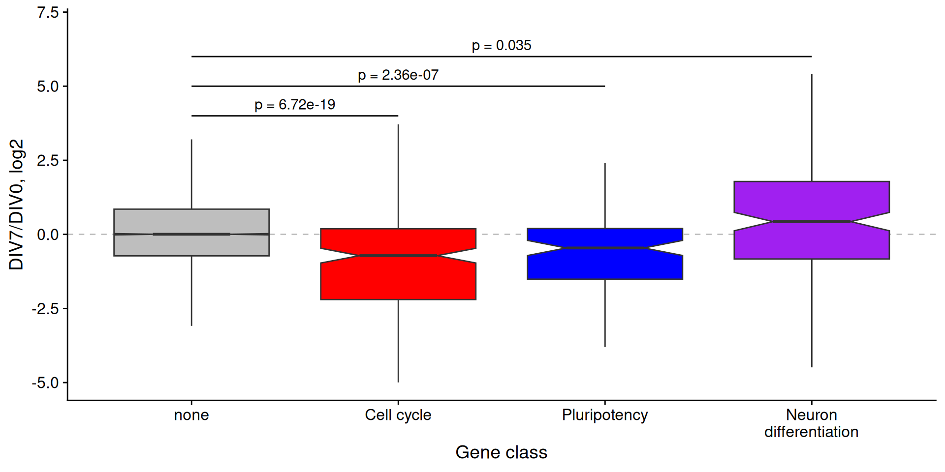
What if we want to look at pathways in an unbiased way?

We will use Gene Set Enrichment Analysis (GSEA) to determine if pre-defined gene sets (pathways, GO terms, experimentally defined genes) are coordinately up-regulated or down-regulated between the two conditions you are comparing. To run gsea you need 2 things. 1. You list of expressed genes ranked by fold change. 2. Pre-defined gene sets. See MSigDb

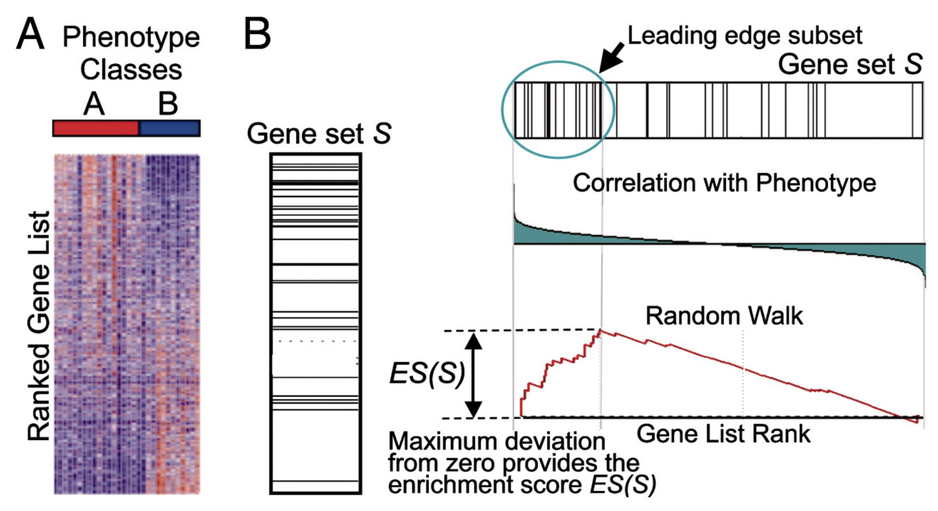
PMID: 12808457, 16199517

GSEA examples

Top = upregulated

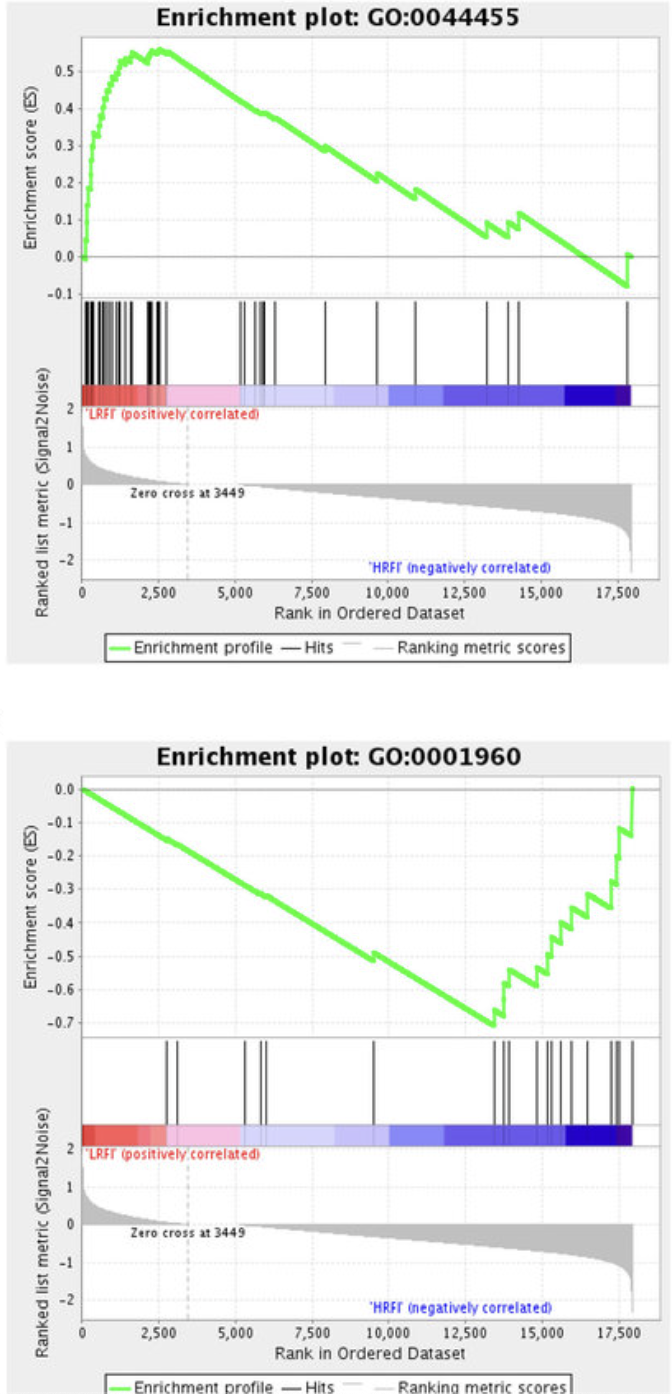
Bottom = downregulated

Prep GSEA

1. We need to make a list of all genes and their LFC.

2. We need to find interesting gene sets.

3. Run GSEA

# retrieve hallmark gene sets from msigdb
mouse_hallmark <- msigdbr(species = "Mus musculus") |>
  filter(gs_collection == "H") |> # "H" is hallmark
  select(gs_name, gene_symbol)

Prep GSEA

Using human MSigDB with ortholog mapping to mouse. Use `db_species = "MM"` for mouse-native gene sets.
Downloading gene sets (first use only, may take a few minutes)...

This message is displayed once per session.

# create a list of gene LFCs
rankedgenes <- diff_lfc |> pull(log2FoldChange)

# add symbols as names of the list
names(rankedgenes) <- diff$gene

# sort by LFC
rankedgenes <- sort(rankedgenes, decreasing = TRUE)

# deduplicate
rankedgenes <- rankedgenes[!duplicated(names(rankedgenes))]

Run GSEA

# rankedgenes[!names(rankedgenes) == ""]

# run gsea
div7vs0 <- GSEA(
  geneList = rankedgenes,
  eps = 0,
  pAdjustMethod = "fdr",
  pvalueCutoff = .05,
  minGSSize = 20,
  maxGSSize = 1000,
  TERM2GENE = mouse_hallmark
)

div7vs0@result |>
  dplyr::select(ID, NES, p.adjust) |>
  gt()

Run GSEA

Plot GSEA

# plot "HALLMARK_G2M_CHECKPOINT"
gseaplot(x = div7vs0, geneSetID = "HALLMARK_G2M_CHECKPOINT")