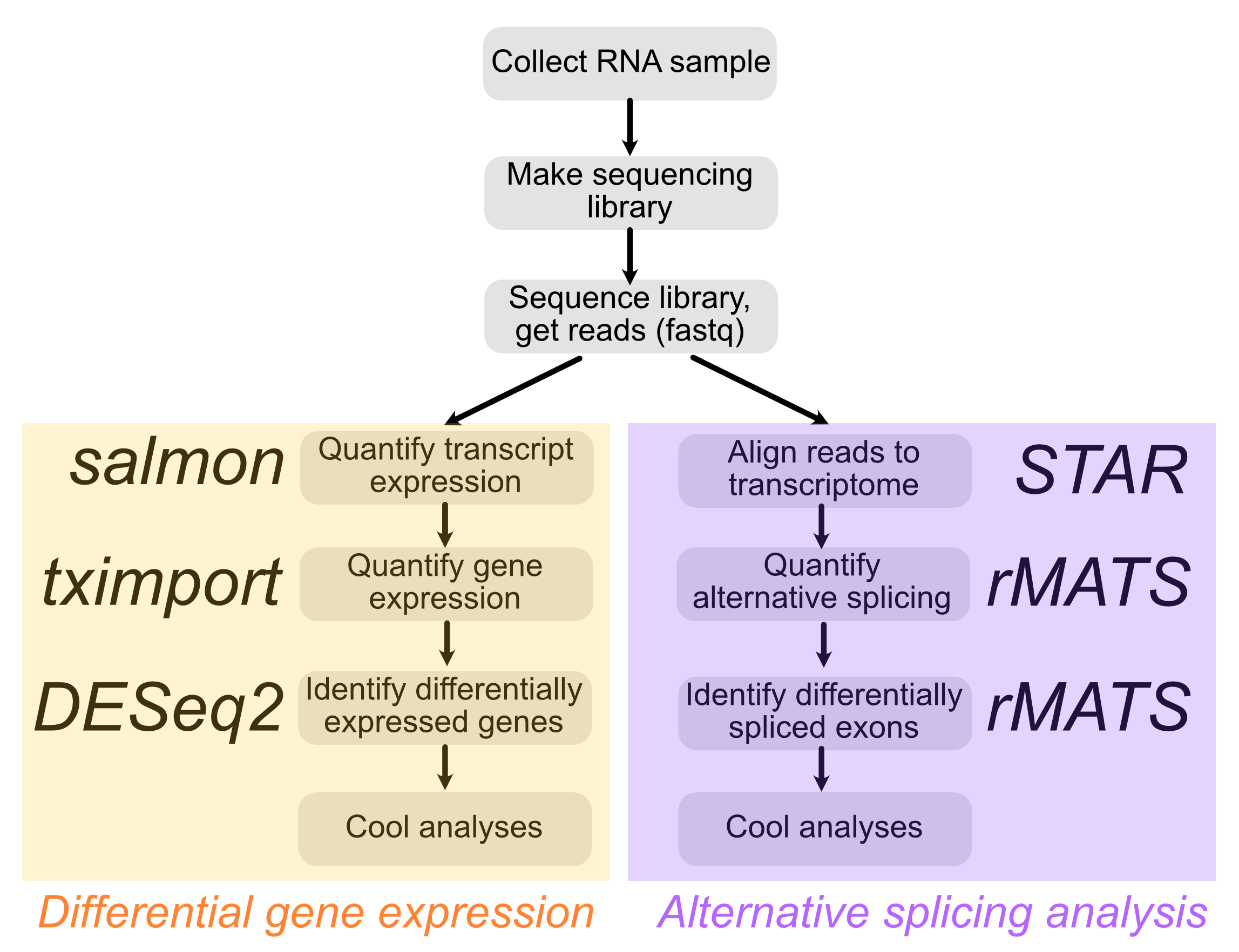
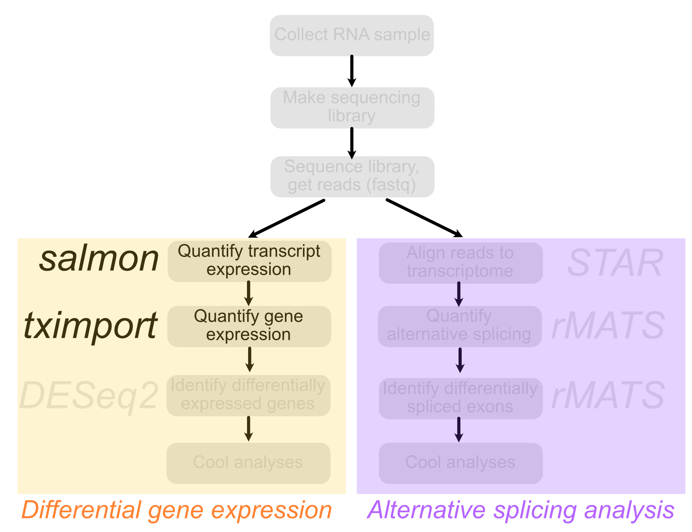
Understand how salmon can be used to quantify gene expression given an RNAseq dataset
Collapse transcript-level quantifications to gene level quantifications using tximport
Deduce the relationships of samples to each other using hierarchical clustering and PCA
Rigor & Reproducibility
As with all computational experiments (yes, they are experiments, don’t let your pipette-toting friends tell you otherwise), keeping track of what you did is key. In the old days, I kept a written notebook of commands that I ran. Sounds silly, but there were many times that I went back to that notebook to see exactly what the parameters were for a given run using a piece of software.
Today, there are better options. You are using one of the better ones right now. Notebooks, including RMarkdown (mainly for R) and Jupyter (mainly for Python), are a great way to keep track of what you did as well as give justification or explanation for your analyses using plain ’ol English.
Trust me, one day you will be glad you used them. The Methods section of your paper is never fun to write without them.
Overview
In this class, we will examine RNAseq data collected over a time-course of differentiation from mouse embryonic stem cells to cortical glutamatergic neurons (Hubbard et al, F1000 Research (2013)). In this publication, the authors differentiated mESCs to neurons using a series of in vitro culture steps over a period of 37 days. During this timecourse, samples were extracted at selected intervals for transcriptome analysis. Importantly, for each timepoint, either 3 or 4 samples were taken for RNA extraction, library preparation and sequencing. This allows us to efficiently use the statistical frameworks provided by the DESeq2 package to identify genes whose RNA expression changes across the timecourse.
Experiment design
Cells were grown in generic differentiation-promoting media (LIF-) for 8 days until aggreates were dissociated and replated in neuronal differentiation media. This day of replating was designated as in vitro day 0 (DIV0). The timepoints taken before this replating therefore happened at “negative” times (DIV-8 and DIV-4). Because naming files with dashes or minus signs can cause problems, these samples are referred to as DIVminus8 and DIVminus4. Following the replating, samples were taken at days 1, 7, 16, 21, and 28 (DIV1, DIV7, DIV16, DIV21, and DIV28).
QC overview
Today we will focus on some quality control steps that are good ideas to do for every RNAseq dataset you encounter, whether produced by yourself or someone else.
Goal
Today we will focus on some Quality Control steps that are good ideas to do for every RNA-seq data set you encounter, whether produced by yourself or someone else.
Quantifying transcript expression with salmon
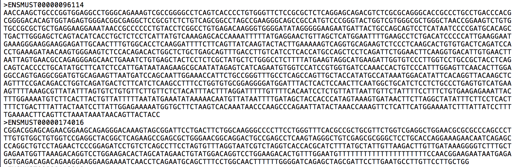
We recently learned about the RNAseq quantification tool salmon. We won’t rehash the details here about how salmon works. For our purposes, we just need to know that salmon reads in a fastq file of sequencing reads and a fasta file of transcript sequences to be quantified. Let’s take a look at this fasta file of transcripts:
Looks like we have ensembl transcript IDs, which is a good idea. I can tell because they start with ‘ENS’. Using ensembl IDs as transcript names will allow us to later collate transcript expression levels into gene expression levels using a database that relates transcripts and genes. More on that later.
Making a transcriptome index
The first step in quantifying these transcripts is to make an index from them. This is done as follows:
salmon index -t<transcripts.fa> -i <transcripts.idx> --type quasi -k<k>
Here, transcripts.fa is a path to our fasta file, transcripts.idx is the name of the index that will be created, and k is the length of the kmers that will be used in the hash table related kmers and transcripts. k is the length of the minimum accepted match for a kmer in a read and a kmer in a transcript. Longer kmers (higher values of k) will therefore be more stringent, and lowering k may improve mapping sensitivity at the cost of some specificity. You may also see here how read lengths can influence what value for k you should choose.
Consider an experiment where we had 25 nt reads (this was true wayyyyyy back in the old, dark days of high-throughput sequencing). What’s going to happen if I quantify these reads using an index where the kmer size was set to 29? Well, nothing will align. The index has represented the transcriptome in 29 nt chunks. However, no read will match to these 29mers because there are no 29mers in these reads! As a general rule of thumb, for reads 75 nt and longer (which is the bulk of the data produced nowadays), a good value for k that maximizes both specificity and sensitivity is 31. However, datasets that you may retrieve from the internet, particularly older ones, may have shorter read lengths, so keep this is mind when defining k.
Quantifying reads against this index
Once we have our index, we can quantify transcripts in the index using reads from our fastq files.
In this command, our forward and reverse read fastq files are supplied to -1 and -2, respectively. If the experiment produced single end reads, -2 is omitted. <transcripts.idx> is the path to the index produced in the previous step. I’m not going to go through the rest of the flags used here, but their meanings as well as other options can be found here.
Salmon outputs
Let’s take a look at what salmon spits out. The first file we will look at is a log that is found at /logs/salmon_quant.log. This file contains info about the quantification, but there’s one line of this file in particular that we are interested in. It lets us know how many of the reads in the fastq file that salmon found a home for in the transcriptome fasta.
less data/block-rna/differentiation_salmonouts/DIV0.Rep1/logs/salmon_quant.log
There are a lot of lines in this file, but really only one that we are interested in. We want the one that tells us the “Mapping rate.” How could we easily and efficiently look at the mapping rates of all our samples? Grep!
#Get the mapping rates for all samples#In each log file, the line that we are interested in contains the string 'Mapping ' (notice the space)grep'Mapping ' data/block-rna/differentiation_salmonouts/*/logs/salmon_quant.log
Moving from transcript quantifications to gene quantifications
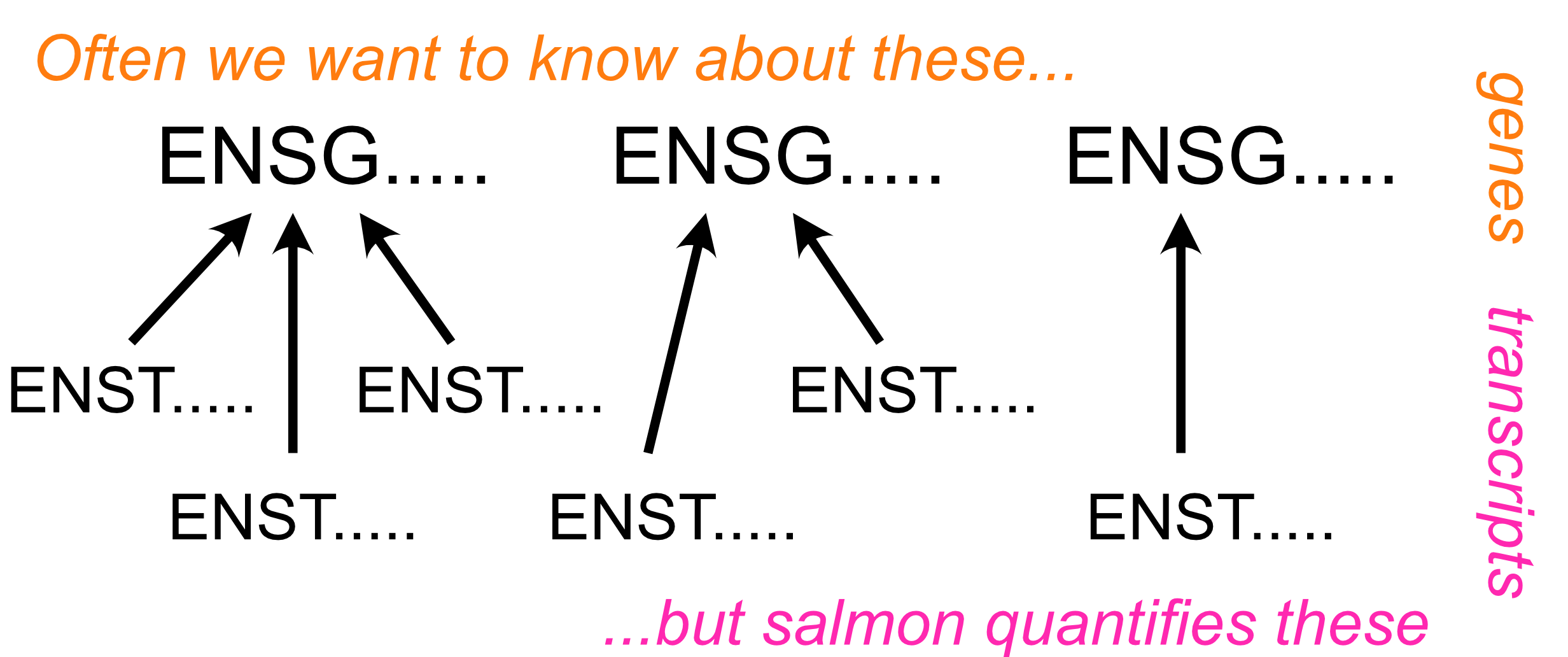
As we discussed, salmon quantifies transcripts, not genes. However, genes are made up of transcripts, so we can calculate gene expression values from transcript expression values if we knew which transcripts belonged to which genes.
Relating genes and transcripts
We can get this relationships between transcripts and genes through AnnotationHub.
AnnotationHub has many tables that relate genes, transcripts, and other useful data including gene biotypes and gene ontology categories, even across species. Let’s use it here to get a table of genes and transcripts for the mouse genome.
ah <-AnnotationHub(ask =FALSE)
# Helper: pull AnnotationHub metadata into a tibble and grab the# most recent EnsDb hit for a given speciesget_latest_ensdb <-function(ah, species) {query(ah, c("EnsDb", species)) |>mcols() |>as_tibble(rownames ="ah_id") |>arrange(desc(rdatadateadded)) |> dplyr::slice(1)}mouse_hit <-get_latest_ensdb(ah, "Mus musculus") |>select(ah_id, title, genome, rdatadateadded)edb_mouse <- ah[[mouse_hit$ah_id]]
downloading 1 resources
retrieving 1 resource
loading from cache
I encourage you to see what is in this database, but for now we are only going to look for transcript IDs and gene IDs.
head(mcols(ah))
DataFrame with 6 rows and 15 columns
                 title dataprovider      species taxonomyid
           <character>  <character>  <character>  <integer>
AH5012 Chromosome Band         UCSC Homo sapiens       9606
AH5013     STS Markers         UCSC Homo sapiens       9606
AH5014     FISH Clones         UCSC Homo sapiens       9606
AH5015     Recomb Rate         UCSC Homo sapiens       9606
AH5016    ENCODE Pilot         UCSC Homo sapiens       9606
AH5017     Map Contigs         UCSC Homo sapiens       9606
            genome            description
       <character>            <character>
AH5012        hg19 GRanges object from ..
AH5013        hg19 GRanges object from ..
AH5014        hg19 GRanges object from ..
AH5015        hg19 GRanges object from ..
AH5016        hg19 GRanges object from ..
AH5017        hg19 GRanges object from ..
       coordinate_1_based             maintainer
                <integer>            <character>
AH5012                  1 Marc Carlson <mcarls..
AH5013                  1 Marc Carlson <mcarls..
AH5014                  1 Marc Carlson <mcarls..
AH5015                  1 Marc Carlson <mcarls..
AH5016                  1 Marc Carlson <mcarls..
AH5017                  1 Marc Carlson <mcarls..
       rdatadateadded          preparerclass
          <character>            <character>
AH5012     2013-03-26 UCSCFullTrackImportP..
AH5013     2013-03-26 UCSCFullTrackImportP..
AH5014     2013-03-26 UCSCFullTrackImportP..
AH5015     2013-03-26 UCSCFullTrackImportP..
AH5016     2013-03-26 UCSCFullTrackImportP..
AH5017     2013-03-26 UCSCFullTrackImportP..
                               tags  rdataclass
                             <AsIs> <character>
AH5012      cytoBand,UCSC,track,...     GRanges
AH5013        stsMap,UCSC,track,...     GRanges
AH5014    fishClones,UCSC,track,...     GRanges
AH5015    recombRate,UCSC,track,...     GRanges
AH5016 encodeRegions,UCSC,track,...     GRanges
AH5017        ctgPos,UCSC,track,...     GRanges
                    rdatapath              sourceurl
                  <character>            <character>
AH5012 goldenpath/hg19/data.. rtracklayer://hgdown..
AH5013 goldenpath/hg19/data.. rtracklayer://hgdown..
AH5014 goldenpath/hg19/data.. rtracklayer://hgdown..
AH5015 goldenpath/hg19/data.. rtracklayer://hgdown..
AH5016 goldenpath/hg19/data.. rtracklayer://hgdown..
AH5017 goldenpath/hg19/data.. rtracklayer://hgdown..
        sourcetype
       <character>
AH5012  UCSC track
AH5013  UCSC track
AH5014  UCSC track
AH5015  UCSC track
AH5016  UCSC track
AH5017  UCSC track
Using AnnotationHub
A lot of stuff for a lot of species! Perhaps we want to limit it to see which ones are relevant to mouse.
Alright this looks good! Although the gene_name field could be useful, for our purposes today, we don’t really need it, and the tools we are using don’t expect it.
Now that we have our table relating transcripts and genes, we can give it to tximport to have it calculate gene-level expression data from our transcript-level expression data.
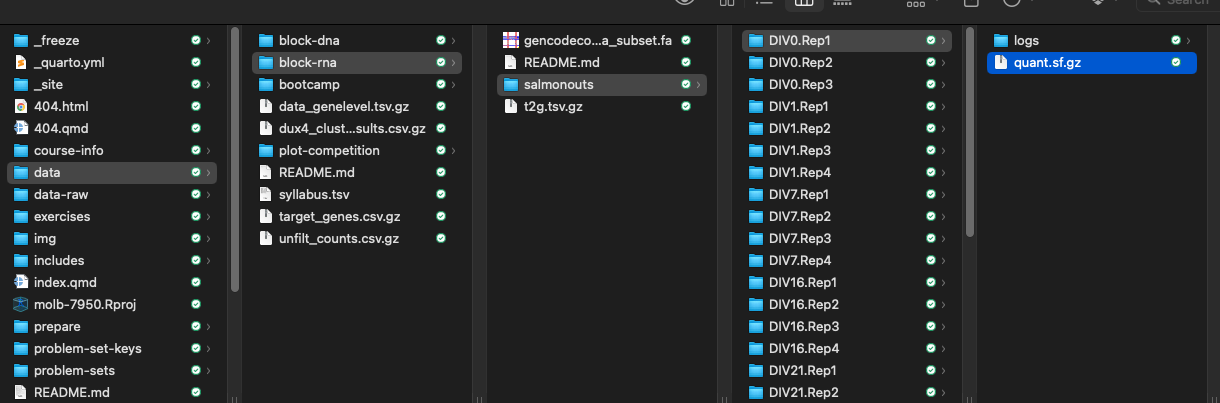
First, we have to tell it where the salmon quantification files (the quant.sf.gz files) are. Here’s what our directory structure that contains these files looks like:
Gene expression data with tximport
# The directory where all of the sample-specific salmon subdirectories livemetadata <-tibble(salmon_dirs = fs::dir_ls(here("data/block-rna/differentiation_salmonouts"),recurse =TRUE,glob ="*quant.sf" )) |>mutate(sample_id = fs::path_file(fs::path_dir(salmon_dirs)) ) |>filter(str_starts(sample_id, "DIV")) |>separate_wider_delim(col = sample_id,delim =".",names =c("samp", "rep"),too_few ="align_start",cols_remove =FALSE ) |>mutate(rep =str_remove(rep, "Rep")) |>column_to_rownames("sample_id")# Add the sample_id column back from rownamesmetadata$sample_id <-rownames(metadata)
Gene expression data with tximport
You can see that we got a list of sample names and the absolute path to each sample’s quantification file.
Now we are ready to run tximport
tximport is going to want paths to all the quantification files (salm_dirs) and a table that relates transcripts to genes (t2g). Luckily, we happen to have those exact two things.
Notice how we chose lengthscaledTPM for our abundance measurement. This is going to give us TPM values (transcripts per million) for expression in the $abundance slot. Let’s check out what we have now.
Let’s stop and think for a minute about what tximport did and the metric we are using (TPM). What does transcripts per million mean? Well, it means pretty much what it sounds like. For every million transcripts in the cell, X of them are this particular transcript. Importantly, this means when this TPM value was calculated from the number of counts a transcript received, this number had to be adjusted for both the total number of counts in the library and the length of a transcript.
If sample A had twice the number of total counts as sample B (i.e. was sequenced twice as deeply), then you would expect every transcript to have approximately twice the number of counts in sample A as it has in sample B. Similarly, if transcript X is twice as long as transcript Y, then you would expect that if they were equally expressed (i.e. the same number of transcript X and transcript Y molecules were present in the sample) that X would have approximately twice the counts that Y does. Working with expression units of TPM incorporates both of these normalizations.
So, if a TPM of X means that for every million transcripts in the sample that X of them were the transcript of interest, then the sum of TPM values across all species should equal one million, right?
Let’s check and see if that’s true.
TPM as an expression metric
sum(tpms$DIVminus8.Rep1)
[1] 985331.8
sum(tpms$DIVminus8.Rep2)
[1] 984957.6
sum(tpms$DIVminus8.Rep3)
[1] 984765.1
OK, not quite one million, but pretty darn close.
This notion that TPMs represent proportions of a whole also leads to another interesting insight into what tximport is doing here. If all transcripts belong to genes, then the TPM for a gene must be the sum of the TPMs of its transcripts. Can we verify that that is true?
TPM as an expression metric
# Redefine for clarity in comparisonstpms.genes <- tpms# Make a new tximport object, but this time instead# of giving gene expression values, give transcript expression values# This is controlled by the `txOut` argumenttxi.transcripts <-tximport( salmdir,type ="salmon",tx2gene = t2g,dropInfReps =TRUE,countsFromAbundance ="lengthScaledTPM",txOut =TRUE)
# Make a table of tpm values for every transcripttpms.txs <-as.data.frame(txi.transcripts$abundance) |>set_names(rownames(metadata)) |>rownames_to_column(var ="ensembl_transcript_id") |>inner_join(t2g, ., by ="ensembl_transcript_id")gt(tpms.txs[1:20, ])
ensembl_transcript_id
DIV0.Rep1
DIV0.Rep2
DIV0.Rep3
DIV1.Rep1
DIV1.Rep2
DIV1.Rep3
DIV1.Rep4
DIV16.Rep1
DIV16.Rep2
DIV16.Rep3
DIV16.Rep4
DIV21.Rep1
DIV21.Rep2
DIV21.Rep3
DIV21.Rep4
DIV28.Rep1
DIV28.Rep2
DIV28.Rep3
DIV28.Rep4
DIV7.Rep1
DIV7.Rep2
DIV7.Rep3
DIV7.Rep4
DIVminus4.Rep1
DIVminus4.Rep2
DIVminus4.Rep3
DIVminus8.Rep1
DIVminus8.Rep2
DIVminus8.Rep3
DIVminus8.Rep4
ensembl_gene_id
ENSMUST00000119854
2.286511
2.475351
2.778492
3.752931
4.290970
3.606815
2.289835
4.753009
6.407206
6.093523
8.073422
4.114218
3.854100
4.504607
4.233634
0.000000
3.062028
2.657892
4.551532
7.708040
5.771621
4.913897
5.733164
0.821894
0.000000
0.791545
0.452225
0.283685
0.253438
0.000000
ENSMUSG00000037736
ENSMUST00000147408
0.000000
0.000000
0.000000
0.000000
0.000000
0.000000
0.000000
0.000000
0.000000
0.000000
0.000000
0.000000
0.000000
0.000000
0.000000
0.000000
0.000000
0.000000
0.000000
0.000000
0.000000
0.000000
0.000000
0.000000
0.000000
0.000000
0.000000
0.000000
0.000000
0.000000
ENSMUSG00000052516
ENSMUST00000070080
17.294246
16.642412
20.145840
22.849371
23.111531
23.055949
18.922899
85.742059
92.095921
92.061439
90.117232
80.253664
82.962866
82.837521
83.218155
68.286276
59.179619
65.655743
67.027119
61.090866
60.764495
60.258015
58.545413
22.716225
23.042382
25.299848
18.289952
19.497363
17.597384
22.126199
ENSMUSG00000056124
ENSMUST00000033908
0.277638
0.771701
0.734236
0.835938
1.130580
1.774933
0.262763
0.231432
0.209738
0.302866
0.342360
0.394527
0.196355
0.088545
0.170725
0.088308
0.148182
0.037937
0.361527
0.124041
0.411704
0.216135
0.384765
0.627833
0.412680
0.393967
0.177899
0.097658
0.091573
0.404344
ENSMUSG00000031511
ENSMUST00000174016
8.545914
6.122679
4.978280
13.429257
13.448801
13.789999
9.139241
3.772152
6.493719
6.454788
7.620481
3.964981
3.769810
4.272302
4.711036
4.523138
4.025177
6.303732
5.551957
20.404943
18.886851
26.036222
24.703049
15.936284
17.060844
18.859078
9.623711
12.255722
10.591347
2.846295
ENSMUSG00000036036
ENSMUST00000082868
5.240588
7.435392
21.577246
0.000000
0.000000
0.000000
0.000000
0.000000
0.000000
0.000000
0.000000
0.000000
0.000000
0.000000
0.000000
0.000000
0.000000
0.000000
0.000000
0.000000
0.000000
0.000000
0.000000
0.000000
3.157229
8.363363
2.106274
7.631468
4.013754
0.000000
ENSMUSG00000064802
ENSMUST00000187399
0.000000
0.000000
0.000000
0.000000
0.000000
0.000000
0.000000
0.000000
0.000000
0.000000
0.000000
0.000000
0.000000
0.000000
0.000000
0.000000
0.112263
0.000000
0.000000
0.000000
0.000000
0.000000
0.000000
0.000000
0.000000
0.000000
0.000000
0.000000
0.000000
0.000000
ENSMUSG00000090925
ENSMUST00000159512
1.197789
1.783770
1.592837
3.586005
2.904509
3.830286
1.389749
1.361614
1.953179
1.801017
2.061461
2.504494
1.787667
1.311947
1.985731
2.389696
0.801072
1.741500
1.538186
0.880757
2.094465
0.624705
1.609800
0.248865
0.954488
1.411125
1.029973
0.838168
0.218119
0.135338
ENSMUSG00000029207
ENSMUST00000194793
0.000000
0.068955
0.061078
0.064820
0.000000
0.000000
0.000000
0.078959
0.177114
0.299510
0.089493
0.181351
0.080516
0.310951
0.222825
0.324322
0.070346
0.163243
0.468088
0.067476
0.360582
0.332645
0.068630
0.000000
0.000000
0.000000
0.155780
0.076557
0.000000
0.000000
ENSMUSG00000103497
ENSMUST00000221298
0.077941
0.100916
0.090854
0.309668
0.244962
0.239357
0.299259
0.174734
0.291636
0.193253
0.231279
0.296867
0.117060
0.200170
0.109928
0.266300
0.103878
0.301950
0.395391
0.569643
0.215417
0.462677
0.353049
0.000000
0.000000
0.028680
0.000000
0.000000
0.000000
0.050635
ENSMUSG00000113688
ENSMUST00000138551
0.000000
0.000000
0.119676
0.000000
0.000000
0.000000
0.000000
0.000000
0.000000
0.000000
0.000000
0.000000
0.000000
0.000000
0.000000
0.000000
0.000000
0.000000
0.000000
0.000000
0.000000
0.000000
0.000000
0.000000
0.000000
0.000000
0.000000
0.000000
0.000000
0.000000
ENSMUSG00000034164
ENSMUST00000210944
0.000000
0.000000
0.000000
0.000000
0.000000
0.000000
0.000000
0.000000
0.000000
0.000000
0.000000
0.000000
0.000000
0.000000
0.000000
0.000000
0.000000
0.000000
0.000000
0.000000
0.000000
0.000000
0.000000
0.000000
0.000000
0.000000
0.000000
0.000000
0.000000
0.000000
ENSMUSG00000110312
ENSMUST00000194146
0.066535
0.185273
0.055779
0.000000
0.000000
0.000000
0.070382
0.000000
0.000000
0.000000
0.078488
0.000000
0.000000
0.000000
0.000000
0.000000
0.000000
0.000000
0.000000
0.000000
0.129887
0.000000
0.000000
0.000000
0.162839
0.143064
0.000000
0.000000
0.058096
0.000000
ENSMUSG00000102375
ENSMUST00000112725
1.270589
1.049486
1.271776
1.294794
1.619005
1.511612
0.893824
0.688353
0.884466
0.635204
0.709094
0.928998
0.846144
0.829175
0.696928
0.989624
1.018670
0.818393
1.100337
1.270363
0.878781
1.156467
1.281586
1.667594
1.633202
1.868757
1.477511
1.274160
1.640671
1.306233
ENSMUSG00000025269
ENSMUST00000181391
2.222061
1.416381
2.497798
3.006018
3.142753
1.571165
3.167750
3.530355
2.965603
4.649879
3.558337
3.465148
3.203126
3.106205
2.862499
0.000000
1.333758
2.039999
3.282519
5.710520
3.937353
6.847600
3.991743
1.733049
0.496494
1.601051
1.270107
1.507055
1.477476
0.000000
ENSMUSG00000030446
ENSMUST00000223290
0.000000
0.000000
0.000000
0.026984
0.000000
0.000000
0.032844
0.033378
0.000000
0.000000
0.000000
0.000000
0.000000
0.033128
0.000000
0.000000
0.031158
0.072496
0.032133
0.000000
0.031972
0.029910
0.000000
0.000000
0.036096
0.000000
0.029574
0.000000
0.000000
0.000000
ENSMUSG00000035954
ENSMUST00000116191
0.000000
0.044746
0.000000
0.000000
0.104528
0.168647
0.046020
0.048814
0.000000
0.000000
0.000000
0.000000
0.000000
0.000000
0.000000
0.000000
0.000000
0.000000
0.000000
0.000000
0.000000
0.102273
0.042109
0.000000
0.069164
0.000000
0.111104
0.170086
0.000000
0.000000
ENSMUSG00000080078
ENSMUST00000060782
0.267962
0.170311
0.391316
0.446440
0.000000
0.000000
0.389636
0.000000
0.000000
0.000000
0.000000
0.000000
0.000000
0.000000
0.000000
0.000000
0.000000
0.000000
0.000000
0.087233
0.046855
0.000000
0.000000
0.110542
0.000000
0.048208
0.044187
0.083067
0.328807
0.000000
ENSMUSG00000051716
ENSMUST00000141479
0.960027
0.541858
0.000000
0.000000
0.473587
1.080745
0.000000
0.274066
0.000000
0.000000
0.000000
0.000000
0.359059
1.129914
0.300957
0.388096
0.000000
0.000000
0.801308
1.141492
1.285565
0.314952
1.575395
0.000000
0.348874
0.398863
0.000000
0.970236
1.421541
0.351342
ENSMUSG00000049119
ENSMUST00000211096
0.000000
0.000000
0.000000
0.000000
0.000000
0.000000
0.000000
0.000000
0.000000
0.000000
0.000000
0.000000
0.000000
0.000000
0.000000
0.000000
0.000000
0.000000
0.000000
0.000000
0.000000
0.000000
0.000000
0.000000
0.000000
0.000000
0.000000
0.000000
0.000000
0.000000
ENSMUSG00000110353
OK so lets look at the expression of ENSMUSG00000020634 in the first sample (DIVminus8.Rep1).
TPM as an expression metric
# Get sum of tpm values for transcripts that belong to ENSMUSG00000020634tpms.tx.ENSMUSG00000020634 <-filter( tpms.txs, ensembl_gene_id =="ENSMUSG00000020634")sumoftxtpm <-sum(tpms.tx.ENSMUSG00000020634$DIVminus8.Rep1)# Get gene level tpm value of ENSMUSG00000020634genetpm <-filter( tpms.genes, ensembl_gene_id =="ENSMUSG00000020634") |>pull(DIVminus8.Rep1)# Are they the same?sumoftxtpm
[1] 46.71414
genetpm
[1] 46.71414
Basic RNAseq QC
OK now that we’ve got expression values for all genes, we now might want to use these expression values to learn a little bit about our samples. One simple question is > Are replicates similar to each other, or at least more similar to each other than to other samples?
If our data is worth anything at all, we would hope that differences between replicates, which are supposed to be drawn from the same condition, are smaller than differences between samples drawn from different conditions. If that’s not true, it could indicate that one replicate is very different from other replciates (in which case we might want to remove it), or that the data in general is of poor quality.
Another question is:
How similar is each sample to every other sample?
In our timecourse, we might expect that samples drawn from adjacent timepoints might be more similar to each other than samples from more distant timepoints.
Hierarchical clustering
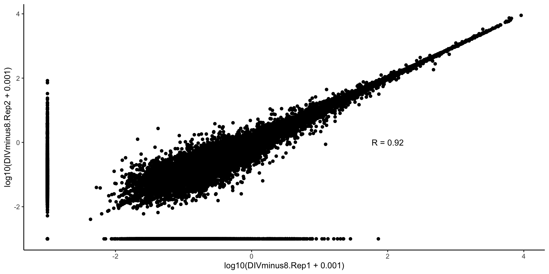
A simple way to think about this is to simply correlate TPM values for genes between samples. For plotting purposes here, let’s plot the log(TPM) of two samples against each other. However, for the actual correlation coefficient we are going to be using the Spearman correlation method, which uses ranks, not absolute values. This means that whether or not you take the log will have no effect on the Spearman correlation coefficient.
# DIVminus8.Rep1 vs DIVminus8.Rep2# Since we are plotting log TPM values, we need to add a pseudocount to all samples.# log(0) is a problem.# Add pseudocounts and take log within ggplot function callr.spearman <-cor.test( tpms$DIVminus8.Rep1, tpms$DIVminus8.Rep2,method ="spearman") |> broom::tidy() |>pull(estimate)
Hierarchical clustering
Warning in cor.test.default(tpms$DIVminus8.Rep1,
tpms$DIVminus8.Rep2, method = "spearman"): Cannot compute
exact p-value with ties
r.spearman <-signif(r.spearman, 2)ggplot( tpms,aes(x =log10(DIVminus8.Rep1 +1e-3), y =log10(DIVminus8.Rep2 +1e-3))) +geom_point() +theme_classic() +annotate("text", x =2, y =0, label =paste0("R = ", r.spearman))
Hierarchical clustering
With RNAseq data, the variance of a gene’s expression increases as the expression increases. However, using a pseudocount and taking the log of the expression value actually reverses this trend. Now, genes with the lowest expression have the most variance. Why is this a problem? Well, the genes with the most variance are going to be the ones that contribute the most to intersample differences. Ideally, we would like to therefore remove the relationship between expression and variance.
There are transformations, notably rlog and vst, that are made to deal with this, but they are best used when dealing with normalized count data, while here we are dealing with TPMs. We will talk about counts later, but not here.
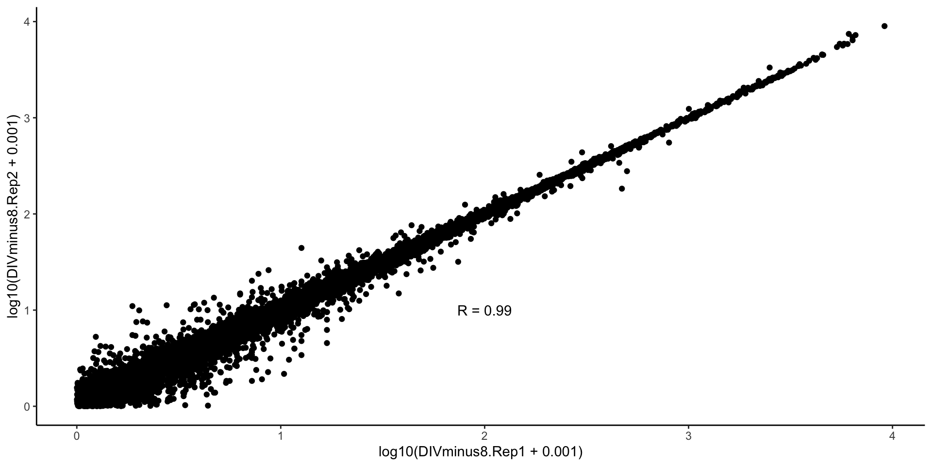
So, for now, we will take another approach of simply using an expression threshold. Any gene that does not meet our threshold will be excluded from the analysis. Obviously where to set this threshold is a bit subjective. For now, we will set this cutoff at 1 TPM.
Hierarchical clustering
# DIVminus8.Rep1 vs DIVminus8.Rep2# Since we are plotting log TPM values we will only keep for genes that have expression of at least 1 TPM in both samplestpms.2samplecor <-select(tpms, c(ensembl_gene_id, DIVminus8.Rep1, DIVminus8.Rep2)) |>filter(DIVminus8.Rep1 >=1& DIVminus8.Rep2 >=1)# pull the correlation coefficientr.spearman <-cor.test( tpms.2samplecor$DIVminus8.Rep1, tpms.2samplecor$DIVminus8.Rep2,method ="spearman") |> broom::tidy() |>pull(estimate)
Hierarchical clustering
Warning in cor.test.default(tpms.2samplecor$DIVminus8.Rep1,
tpms.2samplecor$DIVminus8.Rep2, : Cannot compute exact
p-value with ties
OK that’s two samples compared to each other, but now we want to see how all samples compare to all other samples. Before we do this we need to decide how to apply our expression cutoff across many samples. Should a gene have to meet the cutoff in only one sample? In all samples? Let’s start by saying it has to meet the cutoff in at least half of the 30 samples.
# Make a new column in tpms that is the number of samples in which the value is at least 1tpms.cutoff <-mutate(tpms, nSamples =rowSums(tpms[, 2:31] >1)) |># Now filter for rows where nSamples is at least 15# Meaning that at least 15 samples passed the thresholdfilter(nSamples >=15) |># Get rid of the nSamples columnselect(-nSamples)nrow(tpms)
[1] 49781
nrow(tpms.cutoff)
[1] 14836
Correlating gene expression values
Now we can use the cor function to calculate pairwise correlations in a .red[matrix] of TPM values.
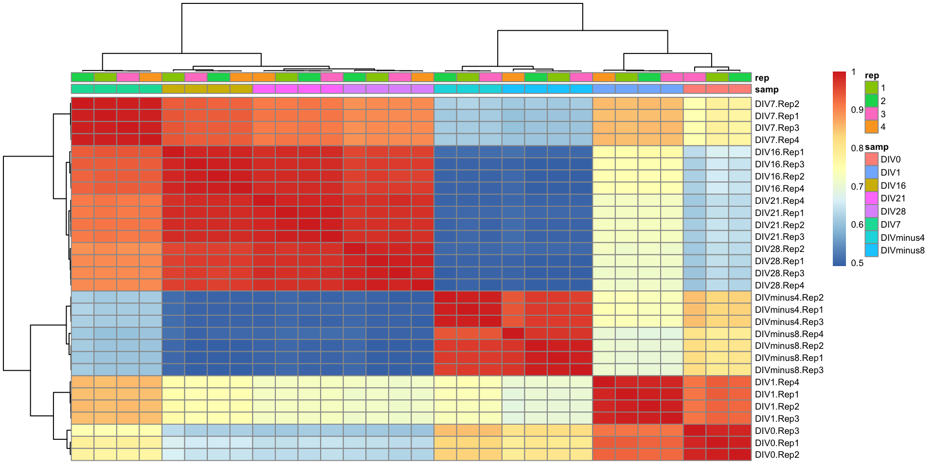
Now we need to plot these and have similar samples (i.e. those that are highly correlated with each other) be clustered near to each other. We will use pheatmap to do this.
# let's pull information that we want to add as categoriespheatmap( tpms.cor,annotation_col = metadata[, 2:3],fontsize =7,show_colnames =FALSE)
This looks pretty good! There are two main points to takeaway here. First, all replicates for a given timepoint are clustering with each other. Second, you can kind of derive the order of the timepoints from the clustering. The biggest separation is between early (DIVminus8 to DIV1) and late (DIV7 to DIV28). After that you can then see finer-grained structure.
Hierarchical clustering
PCA analysis
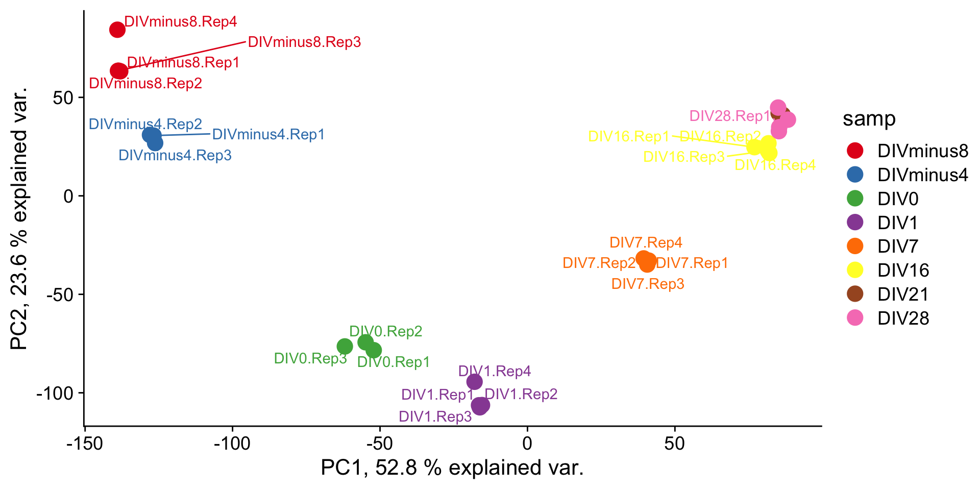
Another way to visualize relationships is using a dimensionality reduction technique called Principal Component Analysis (PCA). Let’s watch this short video. It focuses more on how to interpret them rather than the math behind their creation.
PCA analysis
PCA works best when values are approximately normally distributed, so we will first take the log of our expression values.
With our cutoff as it is now (genes have to have expression of at least 1 TPM in half the samples), it is possible that we will have some 0 values. Taking the log of 0 might cause a problem, so we will add a pseudocount.
tpms.cutoff.matrix <-select(tpms.cutoff, -ensembl_gene_id) |>as.matrix()# Add pseudocount and take log2tpms.cutoff.matrix <-log2(tpms.cutoff.matrix +1e-3)# scale - annoying double transposetpms.cutoff.matrix <-t(scale(t(tpms.cutoff.matrix)))
PCA analysis
Very similar interpretation as before (heatmap of correlation).
# prcomp expects samples to be rownames, right now they are columns# so we need to transpose the matrix using `t`tpms.pca <-prcomp(t(tpms.cutoff.matrix))# The coordinates of samples on the principle components are stored in the $x slot# These are what we are going to use to plot# We can also also some data about the samples here so that our plot is a little more interesting### Tricky piping!!tpms.pca.pc <-as.data.frame(tpms.pca$x) |>rownames_to_column(var ="sample_id") |>left_join(metadata[, 1:4], by ="sample_id")# We can see how much of the total variance is explained by each PC using the summary functiontpms.pca.summary <-summary(tpms.pca)$importance# The amount of variance explained by PC1 is the second row, first column of this table# It's given as a fraction of 1, so we multiply it by 100 to get a percentagepc1var <-round(tpms.pca.summary[2, 1] *100, 1)# The amount of variance explained by PC2 is the second row, second column of this tablepc2var <-round(tpms.pca.summary[2, 2] *100, 1)# Reorder timepoints explicitly for plotting purposestpms.pca.pc$samp <-factor( tpms.pca.pc$samp,levels =c("DIVminus8","DIVminus4","DIV0","DIV1","DIV7","DIV16","DIV21","DIV28" ) )# Plot resultsggplot(data = tpms.pca.pc,aes(x = PC1,y = PC2,color = samp,label = sample_id )) +geom_point(size =5) +scale_color_brewer(palette ="Set1") +theme_cowplot(16) +labs(x =paste("PC1,", pc1var, "% explained var."),y =paste("PC2,", pc2var, "% explained var.") ) +geom_text_repel()