Factor-centric chromatin analysis

Jay Hesselberth

RNA Bioscience Initiative | CU Anschutz

2025-10-20

Where do transcription factors bind in the genome?

Today we’ll look at where two yeast transcription factors bind in the genome using CUT&RUN.

Where do transcription factors bind in the genome?

Techniques like CUT&RUN require an affinity reagent (e.g., an antibody) that uniquely recognizes a transcription factor in the cell.

This antibody is added to permeabilized cells, and the antibody associates with the epitope. A separate reagent, a fusion of Protein A (which binds IgG) and micrococcal nuclease (MNase) then associates with the antibody. Addition of calcium activates MNase, and nearby DNA is digested. These DNA fragments are then isolated and sequenced to identify sites of TF association in the genome.

Where do transcription factors bind in the genome?

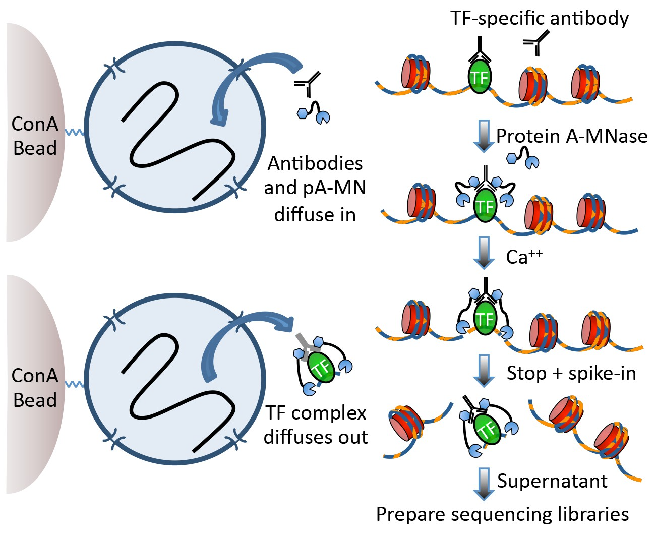
Fig 1a, Skene et al.

Data download and pre-processing

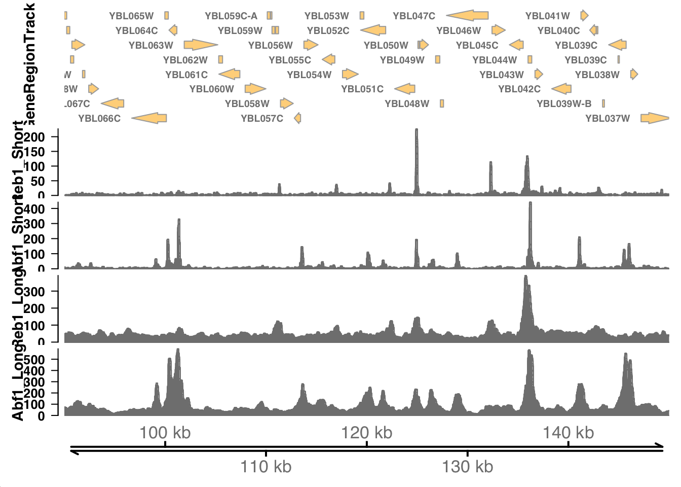
CUT&RUN data were downloaded from the NCBI GEO page for Skene et al.

I selected the 16 second time point for S. cerevisiae Abf1 and Reb1 (note the paper combined data from the 1-32 second time points).

BED files containing mapped DNA fragments were separated by size and converted to bigWig with:

# separate fragments by size
awk '($3 - $2 <= 120)' Abf1.bed > CutRun_Abf1_lt120.bed
awk '($3 - $2 => 150)' Abf1.bed > CutRun_Abf1_gt150.bed

# for each file with the different sizes
bedtools genomecov -i Abf1.bed -g sacCer3.chrom.sizes -bg > Abf1.bg
bedGraphToBigWig Abf1.bg sacCer3.chrom.sizes Abf1.bw

The bigWig files are available here in the data/ directory.

CUT&RUN analysis

library(tidyverse)
library(here)
library(valr)

# genome viz
library(TxDb.Scerevisiae.UCSC.sacCer3.sgdGene)

Warning: replacing previous import
'S4Arrays::makeNindexFromArrayViewport' by
'DelayedArray::makeNindexFromArrayViewport' when loading
'SummarizedExperiment'

library(Gviz)

# motif discovery and viz
library(BSgenome.Scerevisiae.UCSC.sacCer3)
library(memes)
library(ggseqlogo)

track_start <- 90000
track_end <- 150000

# genes track
sgd_genes_trk <-
  GeneRegionTrack(
    TxDb.Scerevisiae.UCSC.sacCer3.sgdGene,
    chromosome = "chrII",
    start = track_start,
    end = track_end,
    background.title = "white",
    col.title = "black",
    fontsize = 16
  )

# signal tracks
track_info <-
  tibble(
    file_name = c(
      "CutRun_Reb1_lt120.bw",
      "CutRun_Abf1_lt120.bw",
      "CutRun_Reb1_gt150.bw",
      "CutRun_Abf1_gt150.bw"
    ),
    sample_type = c(
      "Reb1_Short",
      "Abf1_Short",
      "Reb1_Long",
      "Abf1_Long"
    )
  ) |>
  mutate(
    file_path = here("data/block-dna", file_name),
    big_wig = purrr::map(
      file_path,
      \(x) read_bigwig(x, as = "GRanges")
    ),
    data_track = purrr::map2(
      big_wig,
      sample_type,
      \(x, y) {
        DataTrack(
          x,
          name = y,
          background.title = "white",
          col.title = "black",
          col.axis = "black",
          fontsize = 16
        )
      }
    )
  ) |>
  dplyr::select(sample_type, big_wig, data_track)

# x-axis track
x_axis_trk <- GenomeAxisTrack(
  col = "black",
  col.axis = "black",
  fontsize = 16
)

plotTracks(
  c(
    sgd_genes_trk,
    track_info$data_track,
    x_axis_trk
  ),
  from = track_start,
  to = track_end,
  chromosome = "chrII",
  transcriptAnnotation = "gene",
  shape = "arrow",
  type = "histogram"
)

Genome browser tracks for Abf1 and Reb1 CUT&RUN data.

Peak calling

abf1_tbl <- read_bigwig(here("data/block-dna/CutRun_Abf1_lt120.bw"))
total_reads <- 16e6

genome <- read_genome(here("data/block-dna/sacCer3.chrom.sizes"))
genome_size <- sum(genome$size)

genome_lambda <- total_reads / genome_size
peak_calls <-
  abf1_tbl |>
  # define single-base sites
  mutate(
    midpoint = start + round((end - start) / 2),
    start = midpoint,
    end = start + 1,
    # use the poisson to calculate a p-value with the genome-wide lambda
    pval = dpois(value, genome_lambda),
    # convert p-values to FDR
    fdr = p.adjust(pval, method = "fdr")
  )

Peak calling

peak_calls_sig <-
  filter(
    peak_calls,
    fdr == 0
  ) |>
  # collapse neighboring, significant sites
  bed_merge(max_dist = 20)

filter(
  peak_calls_sig,
  chrom == "chrII" &
    start >= track_start &
    end <= track_end
)

# A tibble: 5 × 3
  chrom  start    end
  <chr>  <int>  <int>
1 chrII 100248 100289
2 chrII 101292 101393
3 chrII 124916 124949
4 chrII 136181 136264
5 chrII 141070 141121

How do proteins recognize specific locations in the genome to bind?

Motif discovery

Theory

There are two major approaches to defining sequence motifs enriched in a sample: enumerative and probabilistic approaches.

Theory

Here we’ll apply a probabilistic approach (MEME) to discover motifs in a collection of DNA sequences. During the RNA block, you’ll learn about k-mer analysis, which is a form of enumerative approach.

In each case, the goal is to define a set of sequence motifs that are encriched in a set of provided sequences (i.e., peaks from CUT&RUN data) relative to a genomic background.

Theory

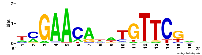
Motifs are expressed in a Position Weight Matrix, which captures the propensities for a position to be a particular nucleotide in a sequence motif.

These PWMs can be represented as sequence logos, visually represent the amount of information provided by the motif, typically using “information content”, expressed in bits.

Theory

LexA sequence motif

Practice

We’ll use the memes package from Bioconductor to derive sequence motifs from the peaks we called above. This is a straightforward process:

Collect the DNA sequences within the peak windows using the BSgenome for S. cerevisiae
Provide those sequences and the genomic background to runDreme(), which runs uses an Expectation-Maximization (EM) approach to identify and refine motifs.
Examine the discovered motifs, and plot as a logo using ggseqlogo.

peak_calls_gr <-
  GRanges(
    seqnames = peak_calls_sig$chrom,
    ranges = IRanges(peak_calls_sig$start, peak_calls_sig$end)
  )

peak_seqs <- BSgenome::getSeq(
  # provided by BSgenome.Scerevisiae.UCSC.sacCer3
  Scerevisiae,
  peak_calls_gr
)

motif_results <- runStreme(
  input = peak_seqs,
  control = "shuffle", # use shuffled sequences as control
  minw = 6, # minimum motif width
  maxw = 12, # maximum motif width
  nmotifs = 5, # number of motifs to find
  seed = 42
)

# look at the consensus motifs
motif_results

Plot the logo

Now let’s look at the sequence logo for the top hit.

motif_1 <- motif_results[[1]]
pwm <- motif_1[[1]]@motif

ggplot() +
  geom_logo(pwm) +
  theme_logo()

Plot the logo

Questions

Does this motif make sense, based on what you know about the requirements and specificity of DNA binding by transcription factors?
How might you confirm that a specific sequence (that conforms to a motif) is bound directly by a transcription factor?