# we are reading the data directly from the internetbiochem <-read_tsv("http://mtweb.cs.ucl.ac.uk/HSMICE/PHENOTYPES/Biochemistry.txt",show_col_types =FALSE) |> janitor::clean_names()# simplify names a bit morecolnames(biochem) <-gsub(pattern ="biochem_",replacement ="",colnames(biochem))# we are going to simplify this a bit and only keep some columnskeep <-colnames(biochem)[c(1, 6, 9, 14, 15, 24:28)]biochem <- biochem[, keep]# get weights for each individual mouse# careful: did not come with column namesweight <-read_tsv("http://mtweb.cs.ucl.ac.uk/HSMICE/PHENOTYPES/weight",col_names = F,show_col_types =FALSE)# add column namescolnames(weight) <-c("subject_name", "weight")# add weight to biochem table and get rid of NAs# rename sex to sexb <-inner_join(biochem, weight, by ="subject_name") |>na.omit() |>rename(sex = gender)
Learning objectives
Formulate and Execute null hypothesis testing
Identify and Perform the proper statistical test for data type/comparison
Calculate and Interpret p-values
Random variables
Response Variable ( y - aka dependent or outcome variable): this variable is predicted or its variation is explained by the explanatory variable. In an experiment, this is the outcome that is measured following manipulation of the explanatory variable.
Explanatory Variable ( x - aka independent or predictor variable): explains variations in the response variable. In an experiment, it is manipulated by the researcher.
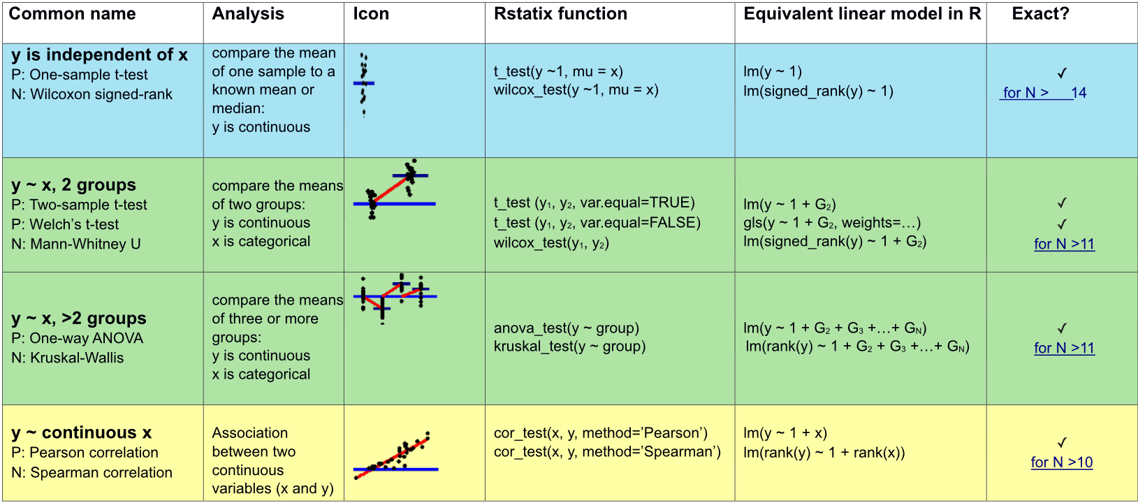
The simplicity underlying common tests
Most of the common statistical models (t-test, correlation, ANOVA; etc.) are special cases of linear models or a very close approximation. This simplicity means that there is less to learn. It all comes down to:
\(y = a \cdot x + b\)
This needless complexity multiplies when students try to rote learn the parametric assumptions underlying each test separately rather than deducing them from the linear model.
Stats equation for a line
Model:
\(y\) equals the intercept (\(\beta_0\)) pluss a slope (\(\beta_1\)) times \(x\).
Since we don’t want to calculate any of this by hand, the framework needs to be flexible such that a computer can execute for different flavors of comparison (cont y vs cont x, cont y vs 2 or more categorical x, …).
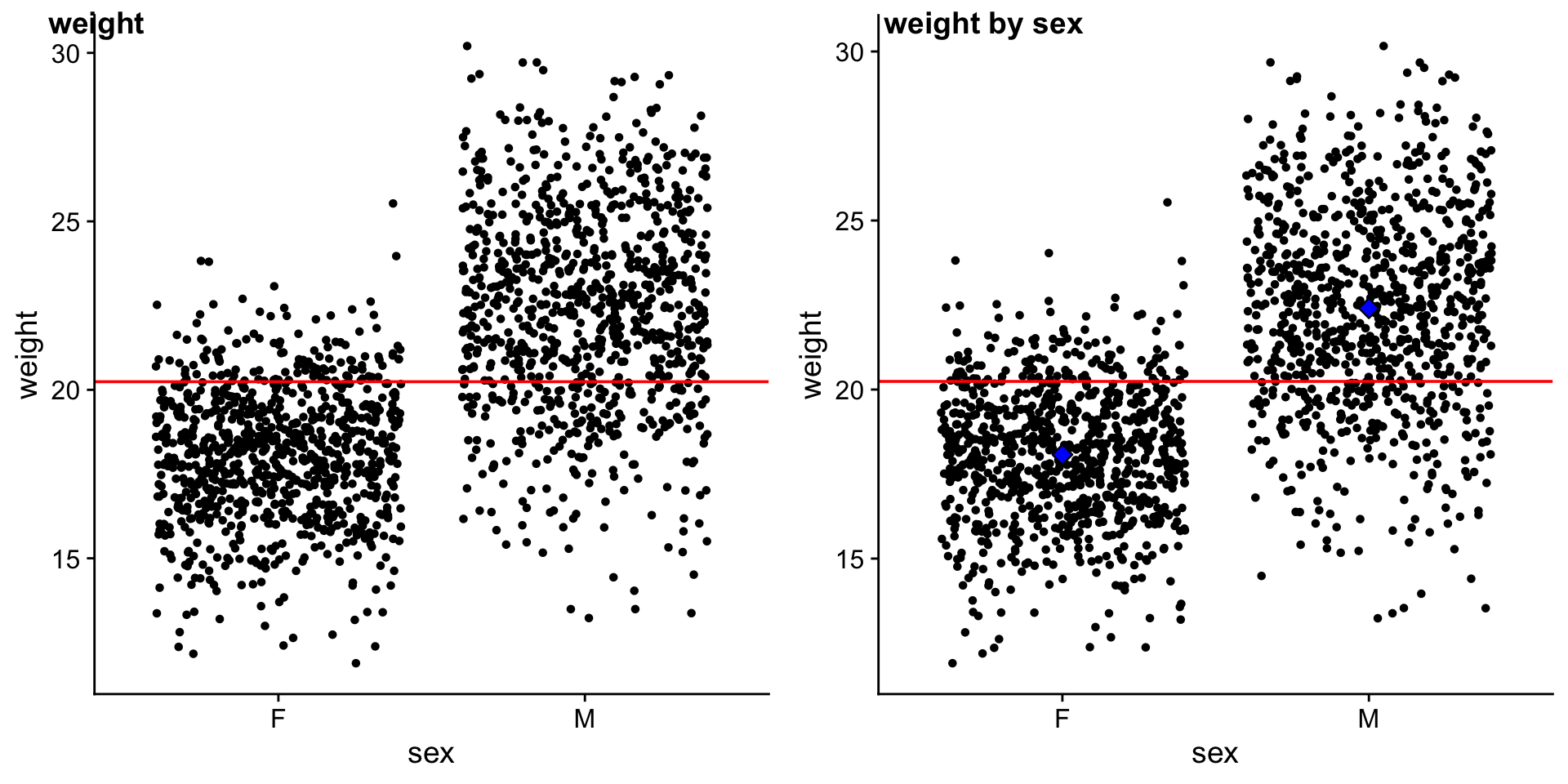
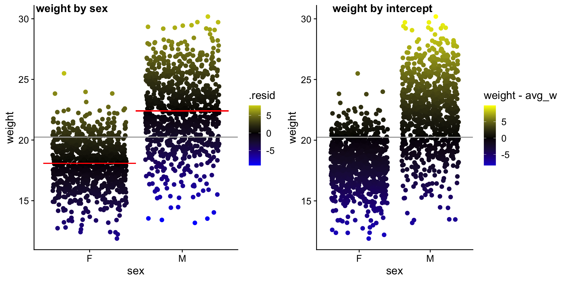
Let’s focus on just a few mice
Remember that: \(weight\) is \(y\) \(F_{avg}\) is the average \(weight\) of \(females\) \(M_{avg}\) is the average \(weight\) of \(males\)
Me: Ooohh my, imagine how tedious it would be to do this for all 1782 mice… Volunteer: Wait a sec…isn’t there a way to formulate this as a matrix algebra problem. Me: You’re right - I’m so glad you asked! Let’s conjur matrix-magic to solve this problem..
\(f_{avg} = \beta_0\) is the average \(weight\) of \(female\) mice \(m_{avg} = \beta_1\) is the average \(weight\) of \(male\) mice
So basically this looks like the same equation for fitting a line we’ve been discussing, just w/a few more dimensions :)
This is a conceptual peak into the underbelly of how the \(\beta\) cofficients and least squares is performed using matrix operations (linear algebra). If you are interested in learning more see references at the end of the slides.
Matrices Interlude FIN
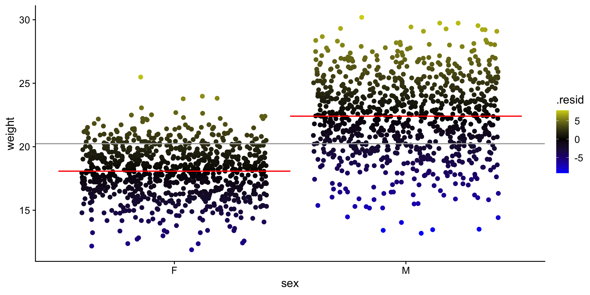
Calculate \(R^2\)
\(SS_{fit}\) — sum of squared errors around the least-squares fit
ss_fit <-sum(b_ws$.resid^2)ss_fit
[1] 11467.91
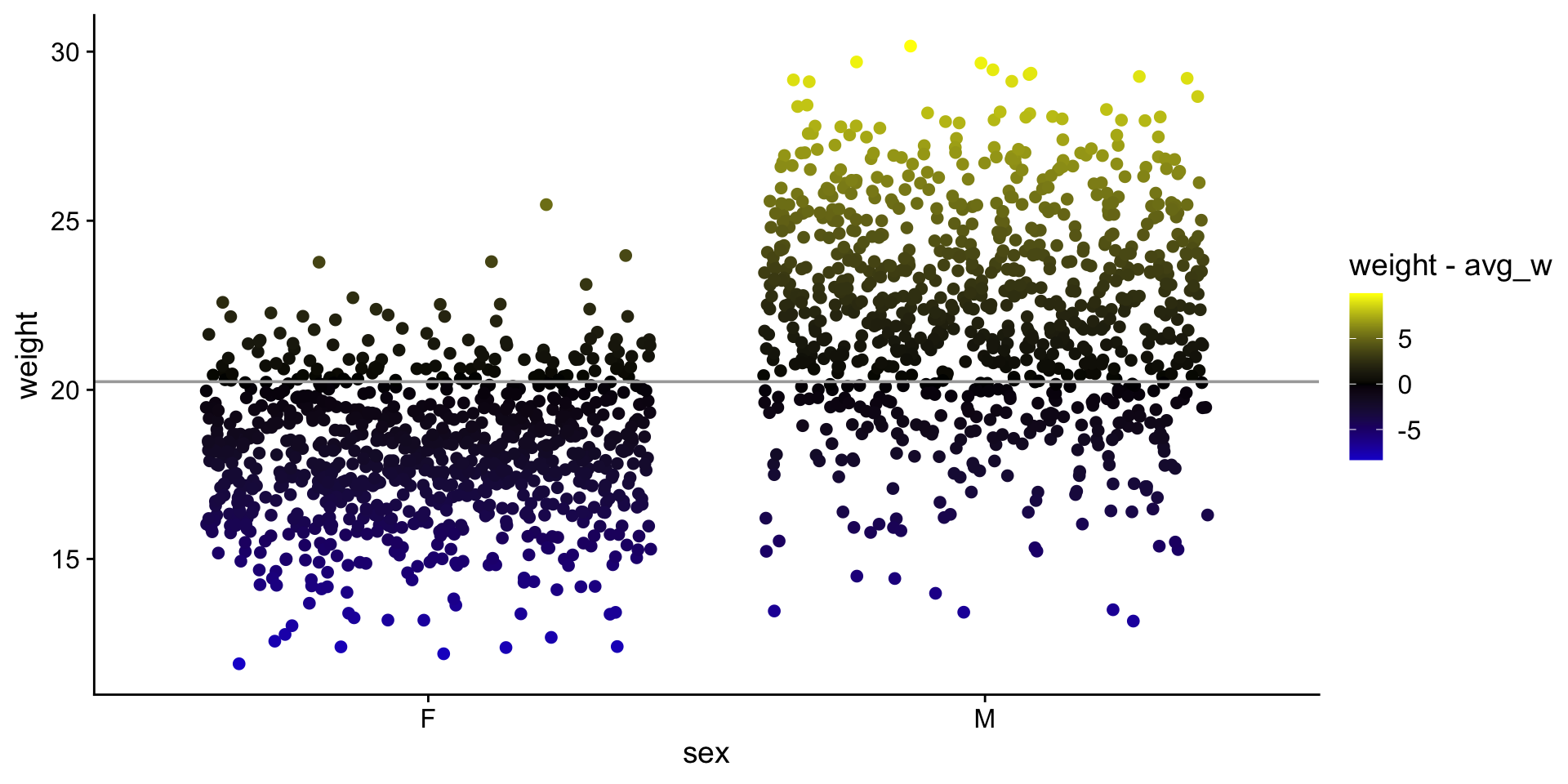
\(SS_{null}\) — sum of squared errors around the mean of \(y\)
# i have pre-selected some families to comparemyfams <-c("B1.5:E1.4(4) B1.5:A1.4(5)","F1.3:A1.2(3) F1.3:E2.2(3)","A1.3:D1.2(3) A1.3:H1.2(3)","D5.4:G2.3(4) D5.4:C4.3(4)")# only keep the familys in myfamsbfam <- b |>filter(family %in% myfams) |>droplevels()# simplify family names and make factorbfam$family <-gsub(pattern ="\\..*", replacement ="", x = bfam$family) |>as.factor()# make B1 the reference (most similar to overall mean)bfam$family <-relevel(x = bfam$family, ref ="B1")
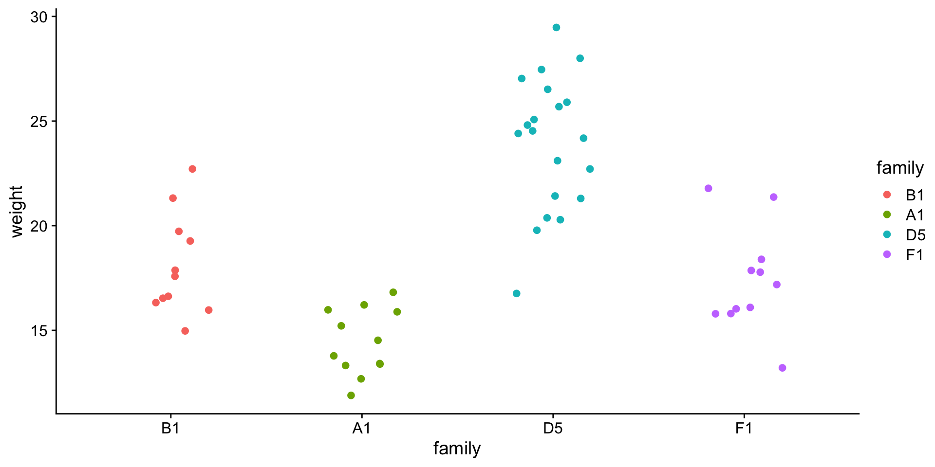
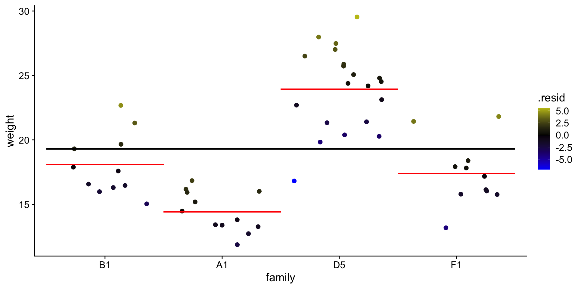
STEP 1: Can family explain weight?
ANOVA -> comparing means of 3 or more groups.
Let’s compare the \(weight\) by \(family\), but only for a few selected families.
ggplot(data = bfam,aes(y = weight, x = family, color = family)) +geom_jitter(width = .2) +theme_cowplot()