R Bootcamp - Day 8

Exercises

Matthew Taliaferro

RNA Bioscience Initiative | CU Anschutz

2026-03-27

R bootcamp review

# import data
data_transcript_exp_tidy <- read_csv(here("data/data_transcript_exp_tidy.csv"))

# save to have smaller name
data <- data_transcript_exp_tidy

# examples of grouping by differently - type these into the console to see the difference
group_by(data, type)

# A tibble: 600 × 5
# Groups:   type [1]
   ensembl_transcript_id      type  time  replicate count
   <chr>                      <chr> <chr> <chr>     <dbl>
 1 ENST00000327044.6_51_2298  rna   0h    rep1        243
 2 ENST00000327044.6_51_2298  rna   0h    rep2        322
 3 ENST00000327044.6_51_2298  rna   0h    rep3        303
 4 ENST00000327044.6_51_2298  rna   14h   rep1        177
 5 ENST00000327044.6_51_2298  rna   14h   rep2        177
 6 ENST00000327044.6_51_2298  rna   14h   rep3        239
 7 ENST00000338591.7_360_2034 rna   0h    rep1         19
 8 ENST00000338591.7_360_2034 rna   0h    rep2         17
 9 ENST00000338591.7_360_2034 rna   0h    rep3         15
10 ENST00000338591.7_360_2034 rna   14h   rep1          9
# ℹ 590 more rows

group_by(data, replicate)

# A tibble: 600 × 5
# Groups:   replicate [3]
   ensembl_transcript_id      type  time  replicate count
   <chr>                      <chr> <chr> <chr>     <dbl>
 1 ENST00000327044.6_51_2298  rna   0h    rep1        243
 2 ENST00000327044.6_51_2298  rna   0h    rep2        322
 3 ENST00000327044.6_51_2298  rna   0h    rep3        303
 4 ENST00000327044.6_51_2298  rna   14h   rep1        177
 5 ENST00000327044.6_51_2298  rna   14h   rep2        177
 6 ENST00000327044.6_51_2298  rna   14h   rep3        239
 7 ENST00000338591.7_360_2034 rna   0h    rep1         19
 8 ENST00000338591.7_360_2034 rna   0h    rep2         17
 9 ENST00000338591.7_360_2034 rna   0h    rep3         15
10 ENST00000338591.7_360_2034 rna   14h   rep1          9
# ℹ 590 more rows

group_by(data, time)

# A tibble: 600 × 5
# Groups:   time [2]
   ensembl_transcript_id      type  time  replicate count
   <chr>                      <chr> <chr> <chr>     <dbl>
 1 ENST00000327044.6_51_2298  rna   0h    rep1        243
 2 ENST00000327044.6_51_2298  rna   0h    rep2        322
 3 ENST00000327044.6_51_2298  rna   0h    rep3        303
 4 ENST00000327044.6_51_2298  rna   14h   rep1        177
 5 ENST00000327044.6_51_2298  rna   14h   rep2        177
 6 ENST00000327044.6_51_2298  rna   14h   rep3        239
 7 ENST00000338591.7_360_2034 rna   0h    rep1         19
 8 ENST00000338591.7_360_2034 rna   0h    rep2         17
 9 ENST00000338591.7_360_2034 rna   0h    rep3         15
10 ENST00000338591.7_360_2034 rna   14h   rep1          9
# ℹ 590 more rows

group_by(data, ensembl_transcript_id)

# A tibble: 600 × 5
# Groups:   ensembl_transcript_id [100]
   ensembl_transcript_id      type  time  replicate count
   <chr>                      <chr> <chr> <chr>     <dbl>
 1 ENST00000327044.6_51_2298  rna   0h    rep1        243
 2 ENST00000327044.6_51_2298  rna   0h    rep2        322
 3 ENST00000327044.6_51_2298  rna   0h    rep3        303
 4 ENST00000327044.6_51_2298  rna   14h   rep1        177
 5 ENST00000327044.6_51_2298  rna   14h   rep2        177
 6 ENST00000327044.6_51_2298  rna   14h   rep3        239
 7 ENST00000338591.7_360_2034 rna   0h    rep1         19
 8 ENST00000338591.7_360_2034 rna   0h    rep2         17
 9 ENST00000338591.7_360_2034 rna   0h    rep3         15
10 ENST00000338591.7_360_2034 rna   14h   rep1          9
# ℹ 590 more rows

# example of how group_by affects the way summarise works
data |> summarise(count = mean(count, na.rm = TRUE))

# A tibble: 1 × 1
  count
  <dbl>
1  144.

group_by(data, time) |> summarise(count = mean(count, na.rm = TRUE))

# A tibble: 2 × 2
  time  count
  <chr> <dbl>
1 0h     185.
2 14h    103.

group_by(data, ensembl_transcript_id) |>
  summarise(count = mean(count, na.rm = TRUE))

# A tibble: 100 × 2
   ensembl_transcript_id          count
   <chr>                          <dbl>
 1 ENST00000054650.8_159_876       8.39
 2 ENST00000054666.10_116_416    121.  
 3 ENST00000054668.5_220_418       3.75
 4 ENST00000234590.8_121_1423   7993.  
 5 ENST00000263741.11_1328_1496   29.4 
 6 ENST00000263741.11_315_1338   141.  
 7 ENST00000270708.11_75_1455     45.7 
 8 ENST00000288774.7_29_1067      16.1 
 9 ENST00000291386.3_370_895     134.  
10 ENST00000307896.10_39_753       8.39
# ℹ 90 more rows

group_by(data, ensembl_transcript_id, time) |>
  summarise(count = mean(count, na.rm = TRUE))

# A tibble: 200 × 3
# Groups:   ensembl_transcript_id [100]
   ensembl_transcript_id        time    count
   <chr>                        <chr>   <dbl>
 1 ENST00000054650.8_159_876    0h       11.3
 2 ENST00000054650.8_159_876    14h       5.5
 3 ENST00000054666.10_116_416   0h      149  
 4 ENST00000054666.10_116_416   14h      93.7
 5 ENST00000054668.5_220_418    0h        0  
 6 ENST00000054668.5_220_418    14h       7.5
 7 ENST00000234590.8_121_1423   0h    10522. 
 8 ENST00000234590.8_121_1423   14h    5465. 
 9 ENST00000263741.11_1328_1496 0h       32.5
10 ENST00000263741.11_1328_1496 14h      26.3
# ℹ 190 more rows

functions to use within mutate - google is your friend
manipulation of cols & rows - use cheatsheets
ggplot
- aesthetic mapping: Ref

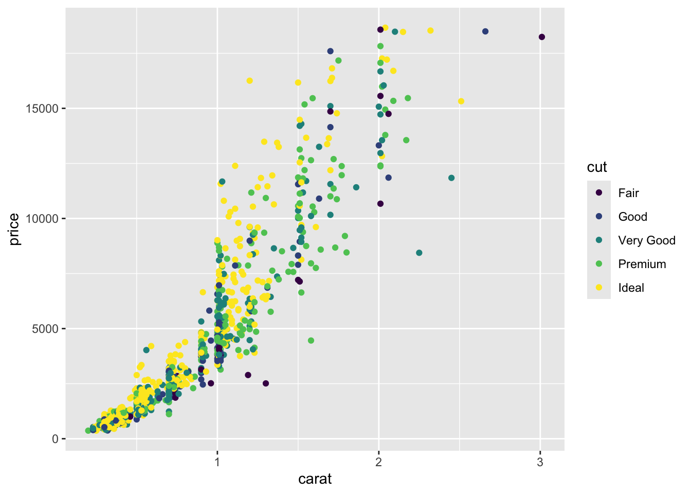
# specifying colors of plots
diamonds_subset <- sample_n(diamonds, size = 1000)

# scatter plot with color by cut - aesthetics specified in the main "mapping"
ggplot(
  diamonds_subset,
  aes(x = carat, y = price, color = cut)
) +
  geom_point()

Description of the plot - PLEASE FILL IN

# scatter plot with color by cut - aesthetics specified in the geom "mapping"
ggplot(
  diamonds_subset,
  aes(x = carat, y = price)
) +
  geom_point(aes(color = cut))

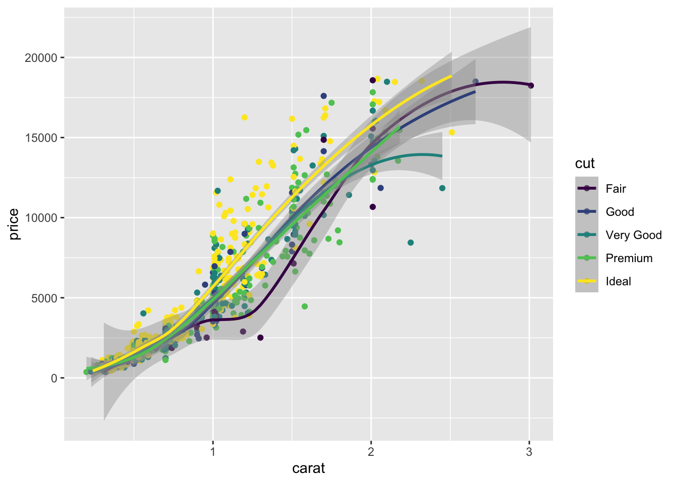
# color specified in the main mapping will apply universally to all geoms
ggplot(
  diamonds_subset,
  aes(x = carat, y = price, color = cut)
) +
  geom_point() +
  geom_smooth()

`geom_smooth()` using method = 'loess' and formula = 'y ~
x'

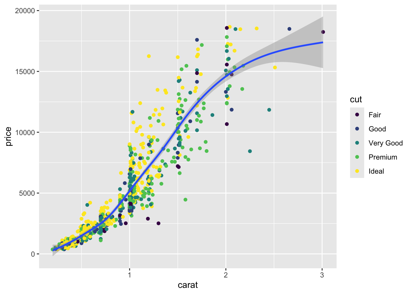
# color specified in the geom mapping only applies to that layer
ggplot(diamonds_subset, mapping = aes(x = carat, y = price)) +
  geom_point(aes(color = cut)) +
  geom_smooth()

`geom_smooth()` using method = 'gam' and formula = 'y ~
s(x, bs = "cs")'

piping data into ggplot - example below

ggplot(
  diamonds_subset,
  aes(x = carat, y = price)
) +
  geom_point(aes(color = cut)) +
  geom_smooth()

`geom_smooth()` using method = 'gam' and formula = 'y ~
s(x, bs = "cs")'

more applied examples - plenty to come in the rest of the course
specifying colors of plots: tutorial

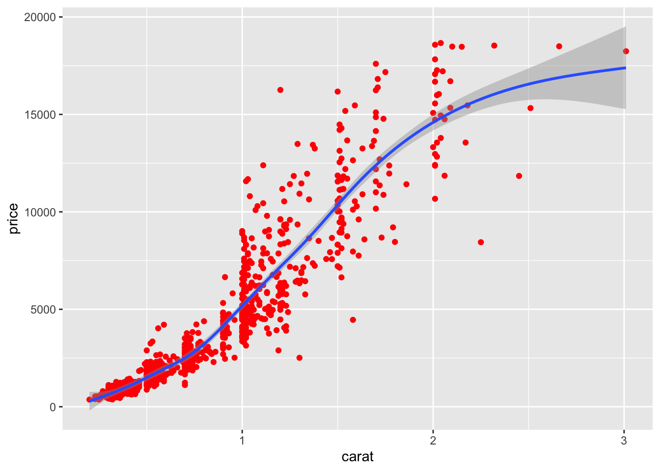
# coloring by a single color - more information in the tutorial above
ggplot(
  data = diamonds_subset,
  mapping = aes(x = carat, y = price)
) +
  geom_point(color = "red") +
  geom_smooth()

`geom_smooth()` using method = 'gam' and formula = 'y ~
s(x, bs = "cs")'

other
- log10 - ?log10
- How to use Help pages: help()
- required vs. optional arguments: this is possible to distinguish if you have a well-documented function. If not, trial-an-error is how it goes.
- Use of commas with multiple vars: Depends on the function. Look at the exact syntax required for specific functions on the cheatsheet to know what to use: col1, col2, col3, vs col1:col3, etc
- Metacharacters “.” etc.: Refer to cheatsheet on Regex + stringr