R Bootcamp - Class 7

tidyverse odds & ends

Matthew Taliaferro

RNA Bioscience Initiative | CU Anschutz

2026-03-27

Class 7 outline

• Accessing data in vectors (Exercise)
• other tidyverse packages (stringr & forcats)
• dplyr table joins (Exercise)
• ggplot2 scale functions
• ggplot2 multi-panel figures (Exercise)
• ggplot2 saving figures

Accessing data in vectors

Using [, [[, and $

# `hp` vector from mtcars
mtcars$hp

 [1] 110 110  93 110 175 105 245  62  95 123 123 180 180 180
[15] 205 215 230  66  52  65  97 150 150 245 175  66  91 113
[29] 264 175 335 109

# columns by name
mtcars[c("hp", "mpg")]

                     hp  mpg
Mazda RX4           110 21.0
Mazda RX4 Wag       110 21.0
Datsun 710           93 22.8
Hornet 4 Drive      110 21.4
Hornet Sportabout   175 18.7
Valiant             105 18.1
Duster 360          245 14.3
Merc 240D            62 24.4
Merc 230             95 22.8
Merc 280            123 19.2
Merc 280C           123 17.8
Merc 450SE          180 16.4
Merc 450SL          180 17.3
Merc 450SLC         180 15.2
Cadillac Fleetwood  205 10.4
Lincoln Continental 215 10.4
Chrysler Imperial   230 14.7
Fiat 128             66 32.4
Honda Civic          52 30.4
Toyota Corolla       65 33.9
Toyota Corona        97 21.5
Dodge Challenger    150 15.5
AMC Javelin         150 15.2
Camaro Z28          245 13.3
Pontiac Firebird    175 19.2
Fiat X1-9            66 27.3
Porsche 914-2        91 26.0
Lotus Europa        113 30.4
Ford Pantera L      264 15.8
Ferrari Dino        175 19.7
Maserati Bora       335 15.0
Volvo 142E          109 21.4

# first 10 items in hp
hp <- mtcars$hp
hp[1:10]

 [1] 110 110  93 110 175 105 245  62  95 123

# 2 ways to get the 10th value
hp[10]
hp[[10]]

# this is an error
hp[[1:10]]

Error in `hp[[1:10]]`:
! attempt to select more than one element in vectorIndex

[ can return a range, [[ returns a single value.

vector selection with logic

one-step filtering.

hp[hp > 100]

 [1] 110 110 110 175 105 245 123 123 180 180 180 205 215 230
[15] 150 150 245 175 113 264 175 335 109

two-step filtering. same result.

# get a vector of T/F values
x <- hp > 100
x

 [1]  TRUE  TRUE FALSE  TRUE  TRUE  TRUE  TRUE FALSE FALSE
[10]  TRUE  TRUE  TRUE  TRUE  TRUE  TRUE  TRUE  TRUE FALSE
[19] FALSE FALSE FALSE  TRUE  TRUE  TRUE  TRUE FALSE FALSE
[28]  TRUE  TRUE  TRUE  TRUE  TRUE

# use that vector to index the original
hp[x]

 [1] 110 110 110 175 105 245 123 123 180 180 180 205 215 230
[15] 150 150 245 175 113 264 175 335 109

also can use with is.na() to identify / exclude NA values in a vector.

Use sum() to figure out how many are TRUE.

x <- hp > 100

# how many are TRUE?
sum(x)

[1] 23

length(hp[x])

[1] 23

other tidyverse libraries

string operations with stringr

stringr provides several useful functions for operating on strings.

See the stringr cheatsheet

str_c("letter: ", letters[1:5])

[1] "letter: a" "letter: b" "letter: c" "letter: d"
[5] "letter: e"

ids <- c("x-1", "x-2", "y-1", "y-2")
str_split(ids, "-")

[[1]]
[1] "x" "1"

[[2]]
[1] "x" "2"

[[3]]
[1] "y" "1"

[[4]]
[1] "y" "2"

# just the first parts
# str_split_i(ids, '-', 1)

str_detect("A", LETTERS[1:5])

[1]  TRUE FALSE FALSE FALSE FALSE

str_pad(
  1:10,
  width = 2,
  side = "left",
  pad = 0
)

 [1] "01" "02" "03" "04" "05" "06" "07" "08" "09" "10"

str_c() is similar to paste and paste0 but the behavior is more consistent.

forcats operations for factors

forcats provides several utilities for working with factors.

See the forcats cheatsheet

library(palmerpenguins)

Attaching package: 'palmerpenguins'

The following objects are masked from 'package:datasets':

    penguins, penguins_raw

penguins[1:3]

# A tibble: 344 × 3
   species island    bill_length_mm
   <fct>   <fct>              <dbl>
 1 Adelie  Torgersen           39.1
 2 Adelie  Torgersen           39.5
 3 Adelie  Torgersen           40.3
 4 Adelie  Torgersen           NA  
 5 Adelie  Torgersen           36.7
 6 Adelie  Torgersen           39.3
 7 Adelie  Torgersen           38.9
 8 Adelie  Torgersen           39.2
 9 Adelie  Torgersen           34.1
10 Adelie  Torgersen           42  
# ℹ 334 more rows

fct_count(penguins$species)

# A tibble: 3 × 2
  f             n
  <fct>     <int>
1 Adelie      152
2 Chinstrap    68
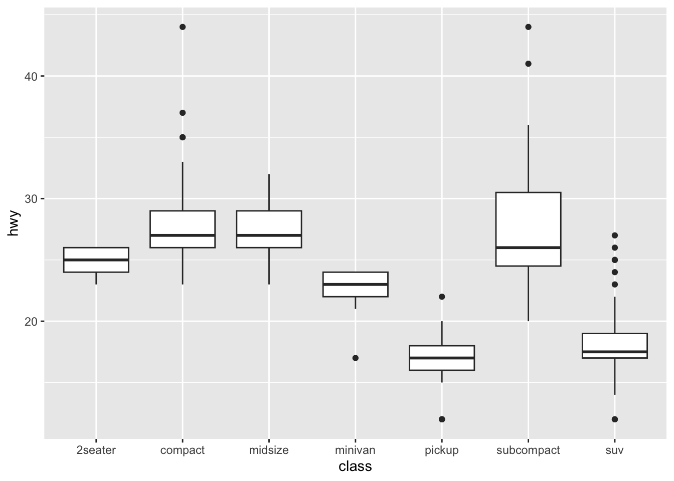
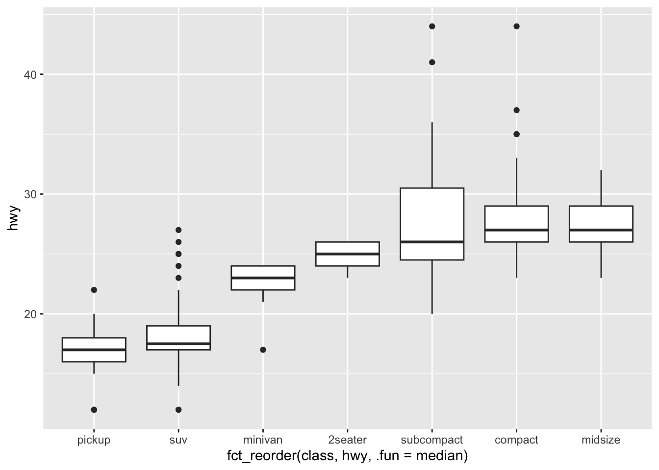
3 Gentoo      124

fct_lump_min(
  penguins$species,
  min = 150
) |>
  fct_count()

# A tibble: 2 × 2
  f          n
  <fct>  <int>
1 Adelie   152
2 Other    192

dplyr::count() is a more flexible alternative to forcats::fct_count()

Use forcats to reorder data in plots

ggplot(
  mpg,
  aes(
    x = class,
    y = hwy
  )
) +
  geom_boxplot()

ggplot(
  mpg,
  aes(
    x = fct_reorder(
      class,
      hwy,
      .fun = median
    ),
    y = hwy
  )
) +
  geom_boxplot()

FAQ on rordering in ggplot2

dplyr

Advanced summarizing with across()

Apply functions to multiple columns at once.

library(palmerpenguins)
penguins |>
  group_by(species) |>
  summarise(
    across(
      c(bill_length_mm, bill_depth_mm, flipper_length_mm),
      list(mean = ~ mean(.x, na.rm = TRUE), sd = ~ sd(.x, na.rm = TRUE))
    ),
    .groups = "drop"
  )

# A tibble: 3 × 7
  species   bill_length_mm_mean bill_length_mm_sd
  <fct>                   <dbl>             <dbl>
1 Adelie                   38.8              2.66
2 Chinstrap                48.8              3.34
3 Gentoo                   47.5              3.08
# ℹ 4 more variables: bill_depth_mm_mean <dbl>,
#   bill_depth_mm_sd <dbl>, flipper_length_mm_mean <dbl>,
#   flipper_length_mm_sd <dbl>

Multiple grouping variables

Complex grouping for detailed analysis.

penguins |>
  group_by(species, island, year) |>
  summarise(
    n_penguins = n(),
    avg_mass = mean(body_mass_g, na.rm = TRUE),
    mass_range = max(body_mass_g, na.rm = TRUE) -
      min(body_mass_g, na.rm = TRUE),
    .groups = "drop"
  ) |>
  arrange(desc(avg_mass))

# A tibble: 15 × 6
   species   island     year n_penguins avg_mass mass_range
   <fct>     <fct>     <int>      <int>    <dbl>      <int>
 1 Gentoo    Biscoe     2009         44    5141.       1625
 2 Gentoo    Biscoe     2007         34    5071.       2200
 3 Gentoo    Biscoe     2008         46    5020.       2050
 4 Adelie    Biscoe     2009         16    3858.       1850
 5 Adelie    Torgersen  2008         16    3856.       1650
 6 Chinstrap Dream      2008         18    3800        2100
 7 Adelie    Torgersen  2007         20    3763.       1475
 8 Adelie    Dream      2008         16    3756.       1550
 9 Chinstrap Dream      2009         24    3725        1200
10 Chinstrap Dream      2007         26    3694.       1500
11 Adelie    Dream      2007         20    3671.       1675
12 Adelie    Dream      2009         20    3651.       1475
13 Adelie    Biscoe     2008         18    3628.       1550
14 Adelie    Biscoe     2007         10    3620         800
15 Adelie    Torgersen  2009         16    3489.       1400

ggplot2

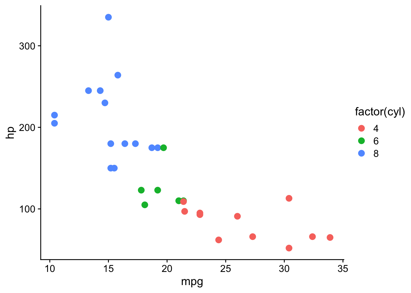
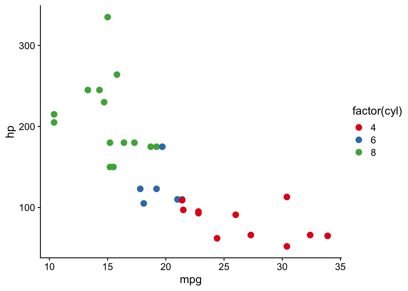
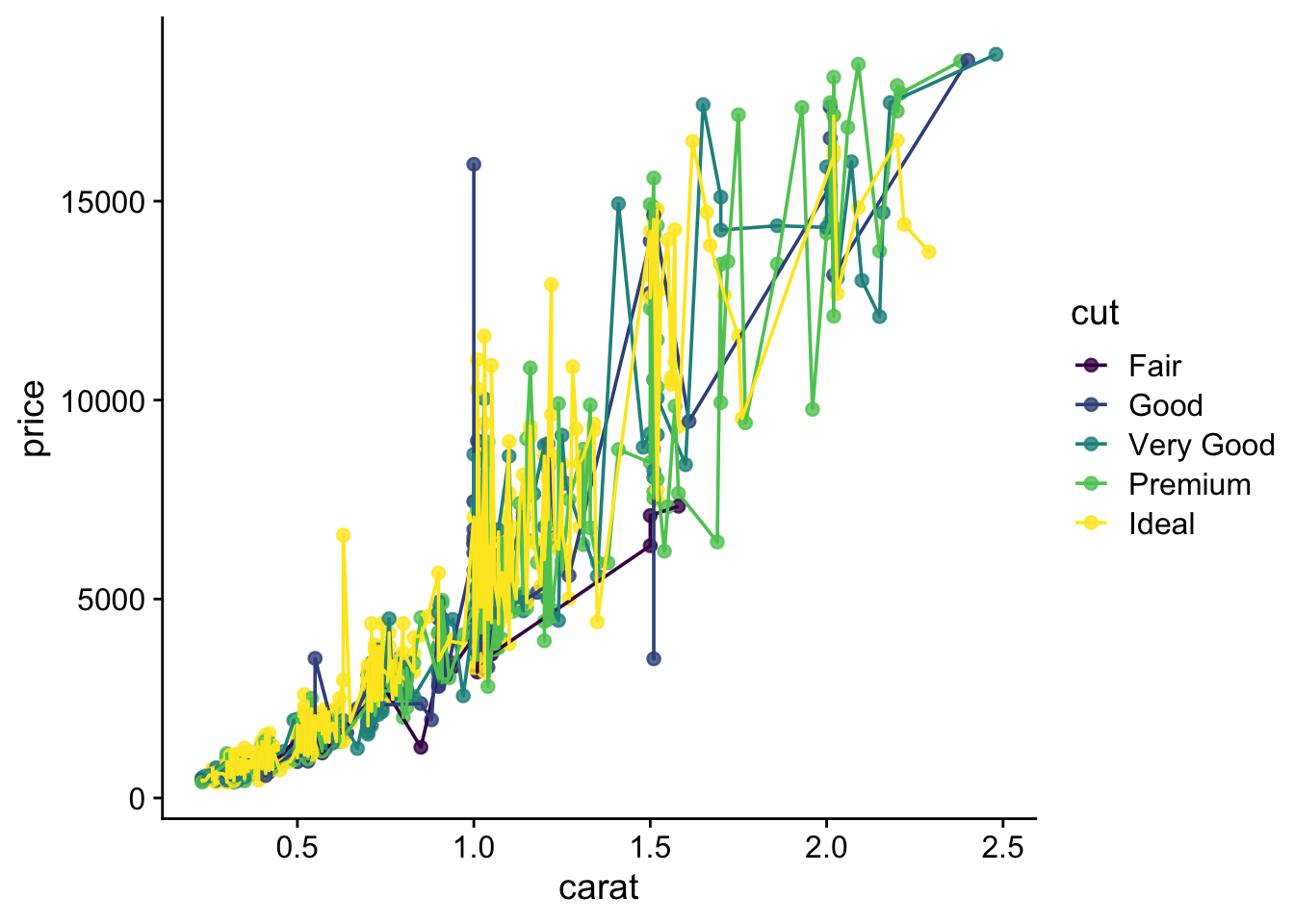
scale functions in ggplot2

• scale_color_brewer() and scale_fill_brewer() control color and fill aesthetics.
• See available ggplot2 brewer palettes

p <- ggplot(
  mtcars,
  aes(
    x = mpg,
    y = hp,
    color = factor(cyl)
  )
) +
  geom_point(size = 3) +
  theme_cowplot()

p

scale functions in ggplot2

p + scale_color_brewer(palette = "Set1")

p + scale_color_brewer(palette = "Dark2")

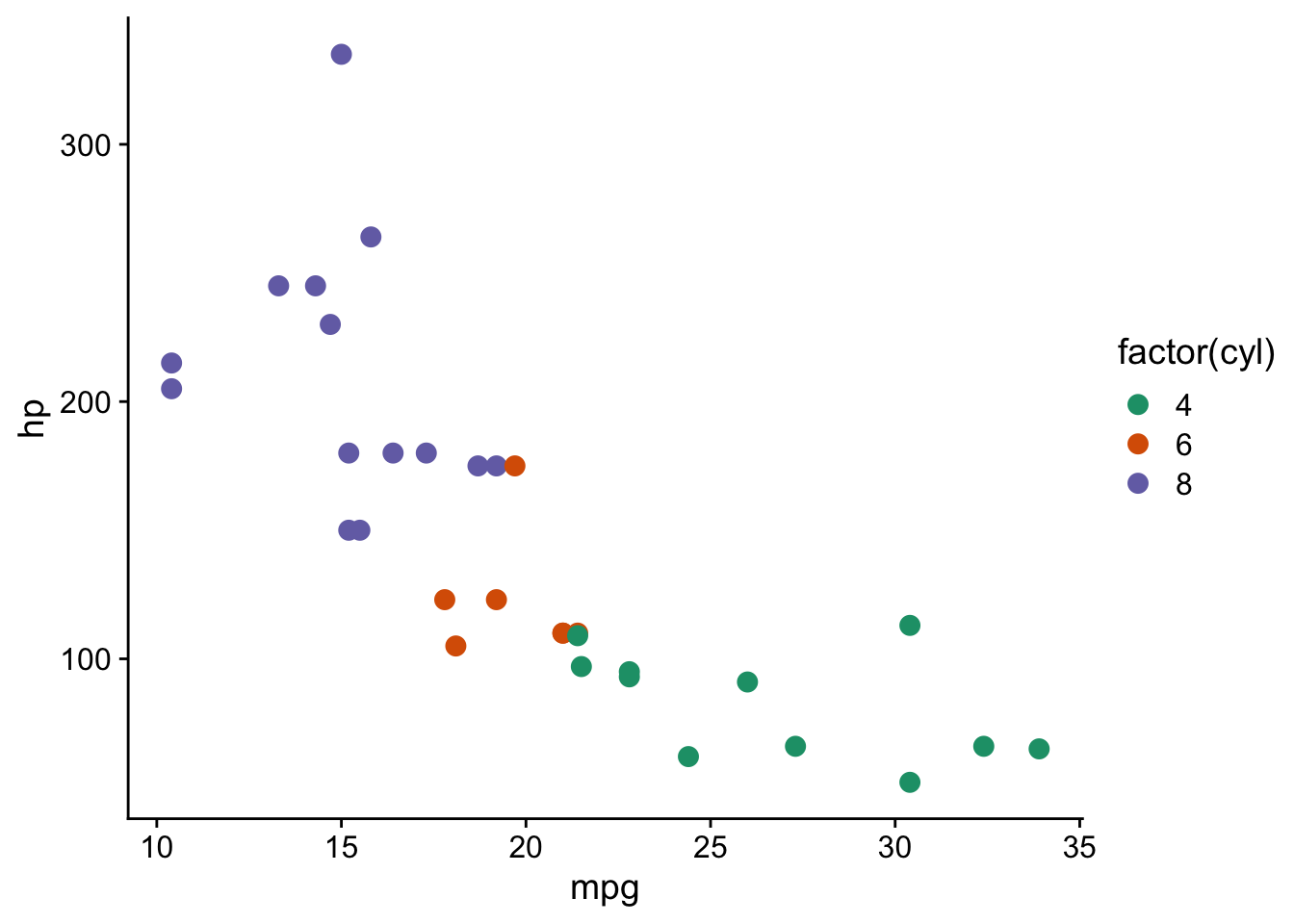
Set up a points plot

diamonds_subset <- sample_n(diamonds, 1000)

p <- ggplot(
  diamonds_subset,
  aes(
    x = carat,
    y = price,
    color = cut
  )
) +
  geom_point(alpha = 0.8) +
  theme_cowplot()

p + geom_line()

How to combine multiple plots into a figure?

# `plot_grid()` is from `cowplot`
plot_grid(
  p,
  p,
  p,
  p,
  labels = c(
    "A",
    "B",
    "C",
    "D"
  ),
  nrow = 2
)

patchwork is a related library that uses arithmetic syntax (a + b | c)

How to combine multiple plots into a figure?

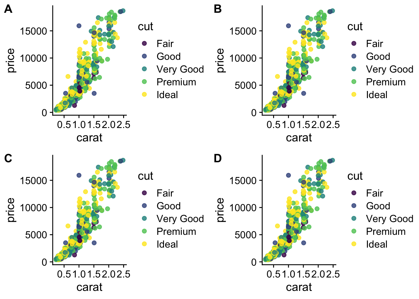
We have 4 legends - can they be condensed?

Yes, but it is not exactly straightforward.

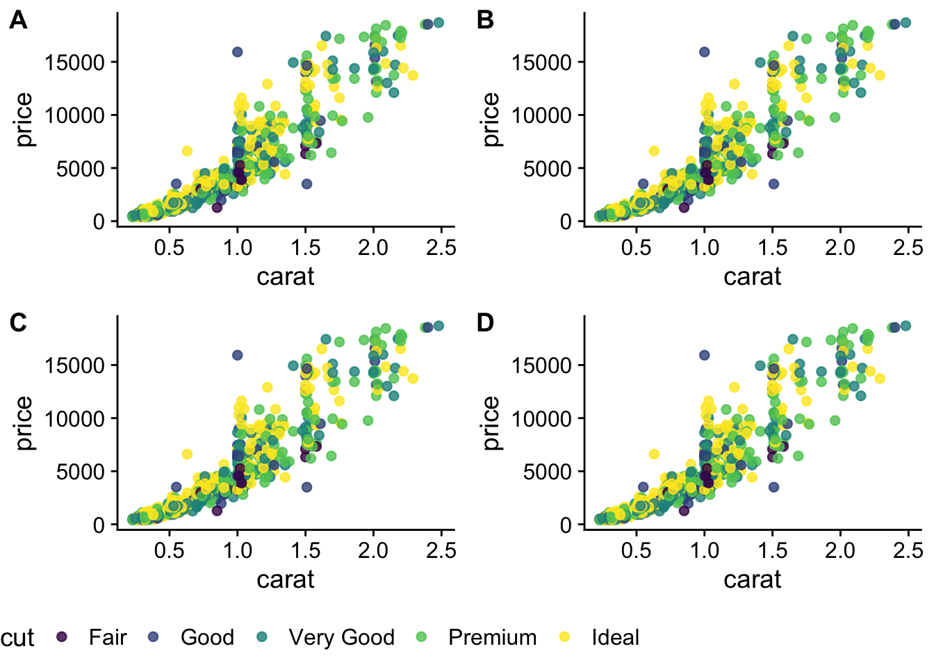
# fetch the legend for `p1`
legend <- get_legend(
  p + theme(legend.position = "bottom")
)

p <- p + theme(legend.position = "none")

# first `plot_grid` builds the panels
panels <- plot_grid(
  p,
  p,
  p,
  p,
  labels = c(
    "A",
    "B",
    "C",
    "D"
  ),
  nrow = 2
)

# second `plot_grid` adds the legend to the panels
plot_grid(
  panels,
  legend,
  ncol = 1,
  rel_heights = c(1, .1)
)

We have 4 legends - can they be condensed?

Saving plots (Exercise 18)

Saves last plot as 5’ x 5’ file named plot_final.png in working directory.

Matches file type to file extension.

# default is to save last plot in the buffer
# can also specify with the `plot` argument
ggsave(
  here("img/plot_final.png"),
  width = 5,
  height = 5
)