R Bootcamp - Day 3

dplyr

Jay Hesselberth

RNA Bioscience Initiative | CU Anschutz

2025-10-20

Class 3 outline

Introduce dplyr & today’s datasets (Exercise 1)
Review basic functions of dplyr
- core dplyr verbs:
- arrange (Exercise 2)
- filter (Exercise 3)
- select (Exercise 4)
- mutate and the pipe (Exercise 5)
- summarise (Exercise 6)
- modify scope of verbs using: group_by (Exercise 7)
- and many others! rename, count, add_row, add_column, distinct, sample_n, sample_frac, slice, pull (Exercise 8)

dplyr overview

dplyr:

provides a set of tools for efficiently manipulating data sets in R.
is extremely fast even with large data sets.
follows the tidyverse grammar and philosophy; human-readable and intuitive
encourages linking of verbs together using pipes |> (or the older %>%)

Today’s datasets

We will use a data set that comes with the dplyr package to explore its functions.
dplyr::starwars contains data for characters from Star Wars.

starwars

# A tibble: 87 × 14
   name         height  mass hair_color skin_color eye_color
   <chr>         <int> <dbl> <chr>      <chr>      <chr>    
 1 Luke Skywal…    172    77 blond      fair       blue     
 2 C-3PO           167    75 <NA>       gold       yellow   
 3 R2-D2            96    32 <NA>       white, bl… red      
 4 Darth Vader     202   136 none       white      yellow   
 5 Leia Organa     150    49 brown      light      brown    
 6 Owen Lars       178   120 brown, gr… light      blue     
 7 Beru Whites…    165    75 brown      light      blue     
 8 R5-D4            97    32 <NA>       white, red red      
 9 Biggs Darkl…    183    84 black      light      brown    
10 Obi-Wan Ken…    182    77 auburn, w… fair       blue-gray
# ℹ 77 more rows
# ℹ 8 more variables: birth_year <dbl>, sex <chr>,
#   gender <chr>, homeworld <chr>, species <chr>,
#   films <list>, vehicles <list>, starships <list>

Explore starwars in the console with head(), View(), and summary().

dplyr package

dplyr is a grammar of data manipulation, providing a consistent set of verbs that help you solve the most common data manipulation challenges:

arrange() changes the ordering of the rows.
filter() picks cases based on their values.
select() picks variables based on their names.
mutate() adds new variables that are functions of existing variables
summarise() reduces multiple values down to a single summary.

These all combine naturally with group_by() which allows you to perform any operation “by group”.
Pipes |> allows different functions to be used together to create a workflow. x |> f(y) turns into f(x, y)

arrange - Syntax

arrange() orders rows by values of one or more columns (low to high).
The desc() helper orders high to low.

arrange(data = ..., <colname>)

arrange - Exercise 2

# default is to arrange in ascending order
arrange(starwars, height)

# A tibble: 87 × 14
   name         height  mass hair_color skin_color eye_color
   <chr>         <int> <dbl> <chr>      <chr>      <chr>    
 1 Yoda             66    17 white      green      brown    
 2 Ratts Tyerel     79    15 none       grey, blue unknown  
 3 Wicket Syst…     88    20 brown      brown      brown    
 4 Dud Bolt         94    45 none       blue, grey yellow   
 5 R2-D2            96    32 <NA>       white, bl… red      
 6 R4-P17           96    NA none       silver, r… red, blue
 7 R5-D4            97    32 <NA>       white, red red      
 8 Sebulba         112    40 none       grey, red  orange   
 9 Gasgano         122    NA none       white, bl… black    
10 Watto           137    NA black      blue, grey yellow   
# ℹ 77 more rows
# ℹ 8 more variables: birth_year <dbl>, sex <chr>,
#   gender <chr>, homeworld <chr>, species <chr>,
#   films <list>, vehicles <list>, starships <list>

arrange - Exercise 2

# arrange in descending order
arrange(starwars, desc(height))

# A tibble: 87 × 14
   name         height  mass hair_color skin_color eye_color
   <chr>         <int> <dbl> <chr>      <chr>      <chr>    
 1 Yarael Poof     264    NA none       white      yellow   
 2 Tarfful         234   136 brown      brown      blue     
 3 Lama Su         229    88 none       grey       black    
 4 Chewbacca       228   112 brown      unknown    blue     
 5 Roos Tarpals    224    82 none       grey       orange   
 6 Grievous        216   159 none       brown, wh… green, y…
 7 Taun We         213    NA none       grey       black    
 8 Rugor Nass      206    NA none       green      orange   
 9 Tion Medon      206    80 none       grey       black    
10 Darth Vader     202   136 none       white      yellow   
# ℹ 77 more rows
# ℹ 8 more variables: birth_year <dbl>, sex <chr>,
#   gender <chr>, homeworld <chr>, species <chr>,
#   films <list>, vehicles <list>, starships <list>

arrange - Exercise 2

# arrange by multiple columns
arrange(starwars, height, mass)

# A tibble: 87 × 14
   name         height  mass hair_color skin_color eye_color
   <chr>         <int> <dbl> <chr>      <chr>      <chr>    
 1 Yoda             66    17 white      green      brown    
 2 Ratts Tyerel     79    15 none       grey, blue unknown  
 3 Wicket Syst…     88    20 brown      brown      brown    
 4 Dud Bolt         94    45 none       blue, grey yellow   
 5 R2-D2            96    32 <NA>       white, bl… red      
 6 R4-P17           96    NA none       silver, r… red, blue
 7 R5-D4            97    32 <NA>       white, red red      
 8 Sebulba         112    40 none       grey, red  orange   
 9 Gasgano         122    NA none       white, bl… black    
10 Watto           137    NA black      blue, grey yellow   
# ℹ 77 more rows
# ℹ 8 more variables: birth_year <dbl>, sex <chr>,
#   gender <chr>, homeworld <chr>, species <chr>,
#   films <list>, vehicles <list>, starships <list>

filter - Syntax

filter() chooses rows/cases where conditions are true.

filter(data = ..., <condition>)

filter - Exercise 3

filter(starwars, skin_color == "light")

# A tibble: 11 × 14
   name         height  mass hair_color skin_color eye_color
   <chr>         <int> <dbl> <chr>      <chr>      <chr>    
 1 Leia Organa     150    49 brown      light      brown    
 2 Owen Lars       178   120 brown, gr… light      blue     
 3 Beru Whites…    165    75 brown      light      blue     
 4 Biggs Darkl…    183    84 black      light      brown    
 5 Lobot           175    79 none       light      blue     
 6 Padmé Amida…    185    45 brown      light      brown    
 7 Cordé           157    NA brown      light      brown    
 8 Dormé           165    NA brown      light      brown    
 9 Raymus Anti…    188    79 brown      light      brown    
10 Rey              NA    NA brown      light      hazel    
11 Poe Dameron      NA    NA brown      light      brown    
# ℹ 8 more variables: birth_year <dbl>, sex <chr>,
#   gender <chr>, homeworld <chr>, species <chr>,
#   films <list>, vehicles <list>, starships <list>

filter - Exercise 3

filter(starwars, height < 150)

# A tibble: 10 × 14
   name         height  mass hair_color skin_color eye_color
   <chr>         <int> <dbl> <chr>      <chr>      <chr>    
 1 R2-D2            96    32 <NA>       white, bl… red      
 2 R5-D4            97    32 <NA>       white, red red      
 3 Yoda             66    17 white      green      brown    
 4 Wicket Syst…     88    20 brown      brown      brown    
 5 Watto           137    NA black      blue, grey yellow   
 6 Sebulba         112    40 none       grey, red  orange   
 7 Ratts Tyerel     79    15 none       grey, blue unknown  
 8 Dud Bolt         94    45 none       blue, grey yellow   
 9 Gasgano         122    NA none       white, bl… black    
10 R4-P17           96    NA none       silver, r… red, blue
# ℹ 8 more variables: birth_year <dbl>, sex <chr>,
#   gender <chr>, homeworld <chr>, species <chr>,
#   films <list>, vehicles <list>, starships <list>

filter - Exercise 3

filter(
  starwars,
  mass > mean(mass, na.rm = TRUE)
)

# A tibble: 10 × 14
   name         height  mass hair_color skin_color eye_color
   <chr>         <int> <dbl> <chr>      <chr>      <chr>    
 1 Darth Vader     202   136 none       white      yellow   
 2 Owen Lars       178   120 brown, gr… light      blue     
 3 Chewbacca       228   112 brown      unknown    blue     
 4 Jabba Desil…    175  1358 <NA>       green-tan… orange   
 5 Jek Tono Po…    180   110 brown      fair       blue     
 6 IG-88           200   140 none       metal      red      
 7 Bossk           190   113 none       green      red      
 8 Dexter Jett…    198   102 none       brown      yellow   
 9 Grievous        216   159 none       brown, wh… green, y…
10 Tarfful         234   136 brown      brown      blue     
# ℹ 8 more variables: birth_year <dbl>, sex <chr>,
#   gender <chr>, homeworld <chr>, species <chr>,
#   films <list>, vehicles <list>, starships <list>

filter - Exercise 3

Filter out cases where hair_color is NA

filter(starwars, is.na(hair_color))

# A tibble: 5 × 14
  name          height  mass hair_color skin_color eye_color
  <chr>          <int> <dbl> <chr>      <chr>      <chr>    
1 C-3PO            167    75 <NA>       gold       yellow   
2 R2-D2             96    32 <NA>       white, bl… red      
3 R5-D4             97    32 <NA>       white, red red      
4 Greedo           173    74 <NA>       green      black    
5 Jabba Desili…    175  1358 <NA>       green-tan… orange   
# ℹ 8 more variables: birth_year <dbl>, sex <chr>,
#   gender <chr>, homeworld <chr>, species <chr>,
#   films <list>, vehicles <list>, starships <list>

filter - Exercise 3

The most frequently used comparison operators are:
>, <, >=, <=, == (equal), != (not equal)
is.na(), !is.na(), and %in% (contained in a vector of cases).

filter(
  starwars,
  skin_color %in% c("light", "fair", "pale")
)

# A tibble: 33 × 14
   name         height  mass hair_color skin_color eye_color
   <chr>         <int> <dbl> <chr>      <chr>      <chr>    
 1 Luke Skywal…    172    77 blond      fair       blue     
 2 Leia Organa     150    49 brown      light      brown    
 3 Owen Lars       178   120 brown, gr… light      blue     
 4 Beru Whites…    165    75 brown      light      blue     
 5 Biggs Darkl…    183    84 black      light      brown    
 6 Obi-Wan Ken…    182    77 auburn, w… fair       blue-gray
 7 Anakin Skyw…    188    84 blond      fair       blue     
 8 Wilhuff Tar…    180    NA auburn, g… fair       blue     
 9 Han Solo        180    80 brown      fair       brown    
10 Wedge Antil…    170    77 brown      fair       hazel    
# ℹ 23 more rows
# ℹ 8 more variables: birth_year <dbl>, sex <chr>,
#   gender <chr>, homeworld <chr>, species <chr>,
#   films <list>, vehicles <list>, starships <list>

# can also store as a named vector and use %in% with the vector
color <- c("light", "fair", "pale")
filter(starwars, skin_color %in% color)

# A tibble: 33 × 14
   name         height  mass hair_color skin_color eye_color
   <chr>         <int> <dbl> <chr>      <chr>      <chr>    
 1 Luke Skywal…    172    77 blond      fair       blue     
 2 Leia Organa     150    49 brown      light      brown    
 3 Owen Lars       178   120 brown, gr… light      blue     
 4 Beru Whites…    165    75 brown      light      blue     
 5 Biggs Darkl…    183    84 black      light      brown    
 6 Obi-Wan Ken…    182    77 auburn, w… fair       blue-gray
 7 Anakin Skyw…    188    84 blond      fair       blue     
 8 Wilhuff Tar…    180    NA auburn, g… fair       blue     
 9 Han Solo        180    80 brown      fair       brown    
10 Wedge Antil…    170    77 brown      fair       hazel    
# ℹ 23 more rows
# ℹ 8 more variables: birth_year <dbl>, sex <chr>,
#   gender <chr>, homeworld <chr>, species <chr>,
#   films <list>, vehicles <list>, starships <list>

Conditions can be combined using & (and), | (or).

filter(
  starwars,
  skin_color == "light" | eye_color == "brown"
)

# A tibble: 25 × 14
   name         height  mass hair_color skin_color eye_color
   <chr>         <int> <dbl> <chr>      <chr>      <chr>    
 1 Leia Organa     150  49   brown      light      brown    
 2 Owen Lars       178 120   brown, gr… light      blue     
 3 Beru Whites…    165  75   brown      light      blue     
 4 Biggs Darkl…    183  84   black      light      brown    
 5 Han Solo        180  80   brown      fair       brown    
 6 Yoda             66  17   white      green      brown    
 7 Boba Fett       183  78.2 black      fair       brown    
 8 Lando Calri…    177  79   black      dark       brown    
 9 Lobot           175  79   none       light      blue     
10 Arvel Crynyd     NA  NA   brown      fair       brown    
# ℹ 15 more rows
# ℹ 8 more variables: birth_year <dbl>, sex <chr>,
#   gender <chr>, homeworld <chr>, species <chr>,
#   films <list>, vehicles <list>, starships <list>

filter(
  starwars,
  skin_color == "light" & eye_color == "brown"
)

# A tibble: 7 × 14
  name          height  mass hair_color skin_color eye_color
  <chr>          <int> <dbl> <chr>      <chr>      <chr>    
1 Leia Organa      150    49 brown      light      brown    
2 Biggs Darkli…    183    84 black      light      brown    
3 Padmé Amidala    185    45 brown      light      brown    
4 Cordé            157    NA brown      light      brown    
5 Dormé            165    NA brown      light      brown    
6 Raymus Antil…    188    79 brown      light      brown    
7 Poe Dameron       NA    NA brown      light      brown    
# ℹ 8 more variables: birth_year <dbl>, sex <chr>,
#   gender <chr>, homeworld <chr>, species <chr>,
#   films <list>, vehicles <list>, starships <list>

select - Syntax

select extracts one or more columns from a table

select(data = ..., <colname>)

select - Exercise 4

# select *only* the variable `hair_color`
select(starwars, hair_color)

# A tibble: 87 × 1
   hair_color   
   <chr>        
 1 blond        
 2 <NA>         
 3 <NA>         
 4 none         
 5 brown        
 6 brown, grey  
 7 brown        
 8 <NA>         
 9 black        
10 auburn, white
# ℹ 77 more rows

select - Exercise 4

# drop the variable `hair_color`
select(starwars, -hair_color)

# A tibble: 87 × 13
   name   height  mass skin_color eye_color birth_year sex  
   <chr>   <int> <dbl> <chr>      <chr>          <dbl> <chr>
 1 Luke …    172    77 fair       blue            19   male 
 2 C-3PO     167    75 gold       yellow         112   none 
 3 R2-D2      96    32 white, bl… red             33   none 
 4 Darth…    202   136 white      yellow          41.9 male 
 5 Leia …    150    49 light      brown           19   fema…
 6 Owen …    178   120 light      blue            52   male 
 7 Beru …    165    75 light      blue            47   fema…
 8 R5-D4      97    32 white, red red             NA   none 
 9 Biggs…    183    84 light      brown           24   male 
10 Obi-W…    182    77 fair       blue-gray       57   male 
# ℹ 77 more rows
# ℹ 6 more variables: gender <chr>, homeworld <chr>,
#   species <chr>, films <list>, vehicles <list>,
#   starships <list>

select - Exercise 4

select(starwars, hair_color, skin_color, eye_color)

# A tibble: 87 × 3
   hair_color    skin_color  eye_color
   <chr>         <chr>       <chr>    
 1 blond         fair        blue     
 2 <NA>          gold        yellow   
 3 <NA>          white, blue red      
 4 none          white       yellow   
 5 brown         light       brown    
 6 brown, grey   light       blue     
 7 brown         light       blue     
 8 <NA>          white, red  red      
 9 black         light       brown    
10 auburn, white fair        blue-gray
# ℹ 77 more rows

select - Exercise 4

# select variables `hair_color` through `eye_color`
select(starwars, hair_color:eye_color)

# A tibble: 87 × 3
   hair_color    skin_color  eye_color
   <chr>         <chr>       <chr>    
 1 blond         fair        blue     
 2 <NA>          gold        yellow   
 3 <NA>          white, blue red      
 4 none          white       yellow   
 5 brown         light       brown    
 6 brown, grey   light       blue     
 7 brown         light       blue     
 8 <NA>          white, red  red      
 9 black         light       brown    
10 auburn, white fair        blue-gray
# ℹ 77 more rows

select - Exercise 4

# drop variables `hair_color` through `eye_color`
select(starwars, !(hair_color:eye_color))

# A tibble: 87 × 11
   name       height  mass birth_year sex   gender homeworld
   <chr>       <int> <dbl>      <dbl> <chr> <chr>  <chr>    
 1 Luke Skyw…    172    77       19   male  mascu… Tatooine 
 2 C-3PO         167    75      112   none  mascu… Tatooine 
 3 R2-D2          96    32       33   none  mascu… Naboo    
 4 Darth Vad…    202   136       41.9 male  mascu… Tatooine 
 5 Leia Orga…    150    49       19   fema… femin… Alderaan 
 6 Owen Lars     178   120       52   male  mascu… Tatooine 
 7 Beru Whit…    165    75       47   fema… femin… Tatooine 
 8 R5-D4          97    32       NA   none  mascu… Tatooine 
 9 Biggs Dar…    183    84       24   male  mascu… Tatooine 
10 Obi-Wan K…    182    77       57   male  mascu… Stewjon  
# ℹ 77 more rows
# ℹ 4 more variables: species <chr>, films <list>,
#   vehicles <list>, starships <list>

select - Exercise 4

# `starts_with`, `ends_with`, `contains`
select(starwars, ends_with("color"))

# A tibble: 87 × 3
   hair_color    skin_color  eye_color
   <chr>         <chr>       <chr>    
 1 blond         fair        blue     
 2 <NA>          gold        yellow   
 3 <NA>          white, blue red      
 4 none          white       yellow   
 5 brown         light       brown    
 6 brown, grey   light       blue     
 7 brown         light       blue     
 8 <NA>          white, red  red      
 9 black         light       brown    
10 auburn, white fair        blue-gray
# ℹ 77 more rows

mutate - Syntax

mutate() to compute new columns

mutate(data = ..., <newcolname> =  funs(<oldcolname>))
mutate(data = ..., <colname>, funs(x))

or with the the pipe |>

Useful when multiple functions act sequentially on a dataframe.

data |>
  mutate(<colname>, funs(x))

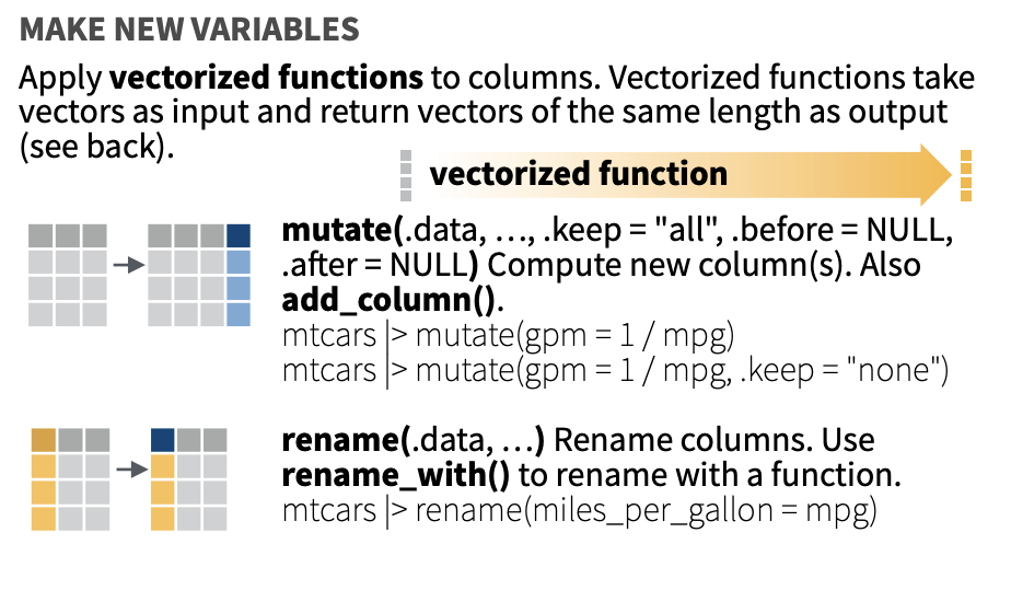
mutate (& pipe |>)- Exercise 5

# create a new column to display height in meters
mutate(starwars, height_m = height / 100)

# A tibble: 87 × 15
   name         height  mass hair_color skin_color eye_color
   <chr>         <int> <dbl> <chr>      <chr>      <chr>    
 1 Luke Skywal…    172    77 blond      fair       blue     
 2 C-3PO           167    75 <NA>       gold       yellow   
 3 R2-D2            96    32 <NA>       white, bl… red      
 4 Darth Vader     202   136 none       white      yellow   
 5 Leia Organa     150    49 brown      light      brown    
 6 Owen Lars       178   120 brown, gr… light      blue     
 7 Beru Whites…    165    75 brown      light      blue     
 8 R5-D4            97    32 <NA>       white, red red      
 9 Biggs Darkl…    183    84 black      light      brown    
10 Obi-Wan Ken…    182    77 auburn, w… fair       blue-gray
# ℹ 77 more rows
# ℹ 9 more variables: birth_year <dbl>, sex <chr>,
#   gender <chr>, homeworld <chr>, species <chr>,
#   films <list>, vehicles <list>, starships <list>,
#   height_m <dbl>

mutate (& pipe |>)- Exercise 5

# using the pipe to feed data into multiple functions sequentially
starwars |>
  mutate(height_m = height / 100) |>
  select(name, height_m, height, everything())

# A tibble: 87 × 15
   name          height_m height  mass hair_color skin_color
   <chr>            <dbl>  <int> <dbl> <chr>      <chr>     
 1 Luke Skywalk…     1.72    172    77 blond      fair      
 2 C-3PO             1.67    167    75 <NA>       gold      
 3 R2-D2             0.96     96    32 <NA>       white, bl…
 4 Darth Vader       2.02    202   136 none       white     
 5 Leia Organa       1.5     150    49 brown      light     
 6 Owen Lars         1.78    178   120 brown, gr… light     
 7 Beru Whitesu…     1.65    165    75 brown      light     
 8 R5-D4             0.97     97    32 <NA>       white, red
 9 Biggs Darkli…     1.83    183    84 black      light     
10 Obi-Wan Keno…     1.82    182    77 auburn, w… fair      
# ℹ 77 more rows
# ℹ 9 more variables: eye_color <chr>, birth_year <dbl>,
#   sex <chr>, gender <chr>, homeworld <chr>,
#   species <chr>, films <list>, vehicles <list>,
#   starships <list>

mutate (& pipe |>)- Exercise 5

Mutate allows you to refer to columns that you’ve just created

starwars |>
  mutate(
    height_m = height / 100,
    BMI = mass / (height_m^2)
  ) |>
  select(name, BMI, everything())

# A tibble: 87 × 16
   name     BMI height  mass hair_color skin_color eye_color
   <chr>  <dbl>  <int> <dbl> <chr>      <chr>      <chr>    
 1 Luke …  26.0    172    77 blond      fair       blue     
 2 C-3PO   26.9    167    75 <NA>       gold       yellow   
 3 R2-D2   34.7     96    32 <NA>       white, bl… red      
 4 Darth…  33.3    202   136 none       white      yellow   
 5 Leia …  21.8    150    49 brown      light      brown    
 6 Owen …  37.9    178   120 brown, gr… light      blue     
 7 Beru …  27.5    165    75 brown      light      blue     
 8 R5-D4   34.0     97    32 <NA>       white, red red      
 9 Biggs…  25.1    183    84 black      light      brown    
10 Obi-W…  23.2    182    77 auburn, w… fair       blue-gray
# ℹ 77 more rows
# ℹ 9 more variables: birth_year <dbl>, sex <chr>,
#   gender <chr>, homeworld <chr>, species <chr>,
#   films <list>, vehicles <list>, starships <list>,
#   height_m <dbl>

Output needs to be saved into a new data frame since dplyr does not “change” the original dataframe.

starwars_bmi <- starwars |>
  mutate(
    height_m = height / 100,
    BMI = mass / (height_m^2)
  ) |>
  select(name, BMI, everything())

`count()` - Count observations

count() is a shortcut for group_by() + summarise() + n().

# Count observations by species
starwars |>
  count(species)

# A tibble: 38 × 2
   species       n
   <chr>     <int>
 1 Aleena        1
 2 Besalisk      1
 3 Cerean        1
 4 Chagrian      1
 5 Clawdite      1
 6 Droid         6
 7 Dug           1
 8 Ewok          1
 9 Geonosian     1
10 Gungan        3
# ℹ 28 more rows

Sort counts with sort = TRUE

# Most common species first
starwars |>
  count(species, sort = TRUE)

# A tibble: 38 × 2
   species      n
   <chr>    <int>
 1 Human       35
 2 Droid        6
 3 <NA>         4
 4 Gungan       3
 5 Kaminoan     2
 6 Mirialan     2
 7 Twi'lek      2
 8 Wookiee      2
 9 Zabrak       2
10 Aleena       1
# ℹ 28 more rows

Count by multiple variables

# Count by species and gender
starwars |>
  count(species, gender, sort = TRUE)

# A tibble: 42 × 3
   species  gender        n
   <chr>    <chr>     <int>
 1 Human    masculine    26
 2 Human    feminine      9
 3 Droid    masculine     5
 4 <NA>     <NA>          4
 5 Gungan   masculine     3
 6 Mirialan feminine      2
 7 Wookiee  masculine     2
 8 Zabrak   masculine     2
 9 Aleena   masculine     1
10 Besalisk masculine     1
# ℹ 32 more rows

count() is equivalent to this longer approach:

# The long way
starwars |>
  group_by(species) |>
  summarise(n = n()) |>
  arrange(desc(n))

# A tibble: 38 × 2
   species      n
   <chr>    <int>
 1 Human       35
 2 Droid        6
 3 <NA>         4
 4 Gungan       3
 5 Kaminoan     2
 6 Mirialan     2
 7 Twi'lek      2
 8 Wookiee      2
 9 Zabrak       2
10 Aleena       1
# ℹ 28 more rows

Complex conditional logic with `case_when()`

starwars |>
  mutate(
    size_description = case_when(
      height < 100 ~ "very short",
      height < 150 ~ "short",
      height < 200 ~ "average",
      height >= 200 ~ "tall",
      .default = "unknown"
    )
  ) |>
  count(size_description)

# A tibble: 5 × 2
  size_description     n
  <chr>            <int>
1 average             60
2 short                3
3 tall                11
4 unknown              6
5 very short           7

Multiple conditions with case_when()

starwars |>
  mutate(
    character_type = case_when(
      species == "Human" & homeworld == "Tatooine" ~ "Tatooine Human",
      species == "Human" ~ "Other Human",
      mass > 100 ~ "Heavy non-human",
      height > 180 ~ "Tall non-human",
      .default = "Standard character"
    )
  ) |>
  count(character_type, sort = TRUE)

# A tibble: 5 × 2
  character_type         n
  <chr>              <int>
1 Other Human           27
2 Standard character    26
3 Tall non-human        18
4 Heavy non-human        8
5 Tatooine Human         8

`group_by()` & `summarise()` - Exercise 6

group_by creates a grouped copy of a table.

This changes the unit of analysis from the complete data set to individual groups.
dplyr verbs automatically detect grouped tables and calculate “by group”.

group_by(data = ..., <colname>)

group_by - Syntax

group_by() creates a grouped tibble.
This changes the unit of analysis from the complete dataset to individual groups.
Then, when you use the dplyr verbs on a grouped data frame they’ll be automatically applied “by group”.

group_by(data = ..., <colname>)

group_by + summarize - Exercise 7

starwars |>
  group_by(species)

# A tibble: 87 × 14
# Groups:   species [38]
   name         height  mass hair_color skin_color eye_color
   <chr>         <int> <dbl> <chr>      <chr>      <chr>    
 1 Luke Skywal…    172    77 blond      fair       blue     
 2 C-3PO           167    75 <NA>       gold       yellow   
 3 R2-D2            96    32 <NA>       white, bl… red      
 4 Darth Vader     202   136 none       white      yellow   
 5 Leia Organa     150    49 brown      light      brown    
 6 Owen Lars       178   120 brown, gr… light      blue     
 7 Beru Whites…    165    75 brown      light      blue     
 8 R5-D4            97    32 <NA>       white, red red      
 9 Biggs Darkl…    183    84 black      light      brown    
10 Obi-Wan Ken…    182    77 auburn, w… fair       blue-gray
# ℹ 77 more rows
# ℹ 8 more variables: birth_year <dbl>, sex <chr>,
#   gender <chr>, homeworld <chr>, species <chr>,
#   films <list>, vehicles <list>, starships <list>

summarize - syntax

summarize() takes named expressions and calculates a summary based on group.

summarize(data = ..., name = expression)

Calculate a summary statistic by species

starwars |>
  group_by(species) |>
  summarise(
    height = mean(height, na.rm = TRUE)
  )

# A tibble: 38 × 2
   species   height
   <chr>      <dbl>
 1 Aleena       79 
 2 Besalisk    198 
 3 Cerean      198 
 4 Chagrian    196 
 5 Clawdite    168 
 6 Droid       131.
 7 Dug         112 
 8 Ewok         88 
 9 Geonosian   183 
10 Gungan      209.
# ℹ 28 more rows

Calucate multiple summary statistics.

starwars |>
  group_by(species, gender) |>
  summarise(
    height = mean(height, na.rm = TRUE),
    mass = mean(mass, na.rm = TRUE)
  )

`summarise()` has grouped output by 'species'. You can
override using the `.groups` argument.

# A tibble: 42 × 4
# Groups:   species [38]
   species   gender    height  mass
   <chr>     <chr>      <dbl> <dbl>
 1 Aleena    masculine     79  15  
 2 Besalisk  masculine    198 102  
 3 Cerean    masculine    198  82  
 4 Chagrian  masculine    196 NaN  
 5 Clawdite  feminine     168  55  
 6 Droid     feminine      96 NaN  
 7 Droid     masculine    140  69.8
 8 Dug       masculine    112  40  
 9 Ewok      masculine     88  20  
10 Geonosian masculine    183  80  
# ℹ 32 more rows

`across()` - Apply functions to multiple columns

across() allows you to apply the same operations to multiple columns efficiently.

# Apply mean to multiple numeric columns
starwars |>
  group_by(species) |>
  summarise(
    across(
      c(height, mass),
      \(x) mean(x, na.rm = TRUE)
    )
  )

# A tibble: 38 × 3
   species   height  mass
   <chr>      <dbl> <dbl>
 1 Aleena       79   15  
 2 Besalisk    198  102  
 3 Cerean      198   82  
 4 Chagrian    196  NaN  
 5 Clawdite    168   55  
 6 Droid       131.  69.8
 7 Dug         112   40  
 8 Ewok         88   20  
 9 Geonosian   183   80  
10 Gungan      209.  74  
# ℹ 28 more rows

R Bootcamp - Day 3

Class 3 outline

dplyr overview

Today’s datasets

dplyr package

arrange - Syntax

arrange - Exercise 2

arrange - Exercise 2

arrange - Exercise 2

filter - Syntax

filter - Exercise 3

filter - Exercise 3

filter - Exercise 3

filter - Exercise 3

filter - Exercise 3

select - Syntax

select - Exercise 4

select - Exercise 4

select - Exercise 4

select - Exercise 4

select - Exercise 4

select - Exercise 4

mutate - Syntax

mutate (& pipe |>)- Exercise 5

mutate (& pipe |>)- Exercise 5

mutate (& pipe |>)- Exercise 5

count() - Count observations

Complex conditional logic with case_when()

group_by() & summarise() - Exercise 6

group_by - Syntax

group_by + summarize - Exercise 7

summarize - syntax

Calculate a summary statistic by species

across() - Apply functions to multiple columns

`count()` - Count observations

Complex conditional logic with `case_when()`

`group_by()` & `summarise()` - Exercise 6

`across()` - Apply functions to multiple columns