Exercises: We want to visualize 1) if RNAs that have HuR binding sites introns, 3’ UTRs, or both exhibit different degrees of stabilization upon HuR knockdown AND 2) which of those categories have a statistically significant different LFC than non-targeted RNAs.
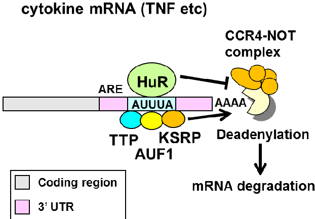
The model we were tesing is that HuR binds to AU-rich elements (ARE) in 3’ UTRs of mRNAs to promote mRNA stability.
This model makes a few specific prediction:
HuR binds to the 3’ UTR and introns.
HuR binds to AU-rich sequences (AUUUA) and U-rich sequences.
HuR binding promotes target RNA stabilization (and binding by the other RBPs to the ARE promotes destabilization).
More specifically, we have been exploring the following questions about the relationship between HuR binding sites and change expression:
Does HuR promote the stability of its mRNA targets?
Does the number of HuR binding influence the degree of stabilization?
Does the region of HuR binding influence stabilization? and Which regions are statistically significant?
We want to visualize 1) if RNAs that have HuR binding sites introns, 3’ UTRs, or both exhibit different degrees of stabilization upon HuR knockdown AND 2) which of those categories have a statistically significant different LFC than non-targeted RNAs. For simplicity, you will categorize genes as either: 1. intron (but not 3’ UTR, ignore other annotation categories)
2. utr3 (but not 3’ intron, ignore other annotation categories)
3. intron and utr3 (ignore other annotation categories) 4. other (genes w/binding sites but none in intron either 3’ UTR)
5. not a target (this is the reference comparison)
1. Annotate HuR binding sites.
1a. Build annotation database
# What annotation categories are available?possible_annotations<-builtin_annotations()# Keep only those containing "hg19"hg19_annots<-grep("hg19_genes", possible_annotations, value =T)# let's keep 5' utr, cds, intron, 3' utr and intergenicmy_hg19_annots<-hg19_annots[c(3, 4, 7, 10, 11)]# build the annotation databaseannotations<-build_annotations(genome ="hg19", annotations =my_hg19_annots)
'select()' returned 1:1 mapping between keys and columns
Building promoters...
Building 1to5kb upstream of TSS...
Building intergenic...
Building cds...
Building 5UTRs...
Building 3UTRs...
Building exons...
Building introns...
1b. Annotate the HuR binding sites
# read hur binding siteshur_regions<-read_regions( con ="https://raw.githubusercontent.com/BIMSBbioinfo/RCAS_meta-analysis/master/rbp-binding-sites/SRR248532.clusters.bed", genome ="hg19", format ="bed")
Attaching package: 'XVector'
The following object is masked from 'package:purrr':

    compact
Attaching package: 'Biostrings'
The following objects are masked from 'package:Hmisc':

    mask, translate
The following object is masked from 'package:base':

    strsplit
# keep only columns we needmyInfo<-c("seqnames","start","end","width","strand","annot.symbol","annot.type")hur_annot<-hur_annot[, myInfo]%>%unique()# getting rid of the "hg19_genes_" string to simplify `annot.type`hur_annot$annot.type<-gsub("hg19_genes_", "", hur_annot$annot.type)
1c. Calculate a summary table for HuR binding sites per gene per region.
Now we want to assemble the # of HuR binding sites per region per gene.
# count the # sites per gene and annotation cathur_gene_clip<-hur_annot%>%filter(annot.type!="intergenic")%>%group_by(annot.symbol, annot.type)%>%dplyr::count()%>%pivot_wider(names_from =annot.type, values_from =n)hur_gene_clip<-hur_gene_clip%>%mutate_if(is.numeric, replace_na, replace =0)
`mutate_if()` ignored the following grouping variables:
• Column `annot.symbol`
# new column w/total # siteshur_gene_clip$total<-rowSums(hur_gene_clip[, -1])# remove symbols that are NAhur_gene_clip<-hur_gene_clip%>%filter(annot.symbol!="NA")# rename colscolnames(hur_gene_clip)[1]<-"Symbol"colnames(hur_gene_clip)[3:4]<-c("utr3", "utr5")# how many genes have both intron and/or 3' UTR sitessite_combo<-hur_gene_clip%>%mutate( type =case_when(introns>0&utr3>0~"intron_utr3",introns>0&utr3==0~"intron",introns==0&utr3>0~"utr3",TRUE~"other"))
1c. import kd data and join w/clip data
# load object called HuR.R# HuR siRNA RNAseqload(here("data/block-rna/HuR.rds"))# gene informationgene_info<-read_csv(here("data/block-rna/geneInfo.csv.zip"))
Multiple files in zip: reading 'geneInfo.csv'
Rows: 63568 Columns: 13
── Column specification ────────────────────────────────────────────────────────
Delimiter: ","
chr (6): Gene, Cat, Annotation, chr, Symbol, strand
dbl (7): row, Exons, Introns, Transcripts, start, end, lengths

ℹ Use `spec()` to retrieve the full column specification for this data.
ℹ Specify the column types or set `show_col_types = FALSE` to quiet this message.
HuR$Gene<-rownames(HuR)# new column gene idsHuR<-left_join(HuR, gene_info[c(2, 11)], by ="Gene")# Symbol# Filter for expressionhur_filt_rnaseq<-HuR%>%dplyr::filter(rowMeans(HuR[, 1:4])>1)%>%dplyr::select(-Gene)kd_clip<-left_join(hur_filt_rnaseq, site_combo, by ="Symbol")# convert all NA to 0kd_clip$type[is.na(kd_clip$type)]<-"not_target"# calculate log fold changes for maturekd_clip<-kd_clip%>%mutate( lfc_mature =log2(Mature_siGFP)-log2(Mature_siHuR))# relevel so "not_target" is refkd_clip$type<-relevel(x =factor(kd_clip$type), ref ="not_target")
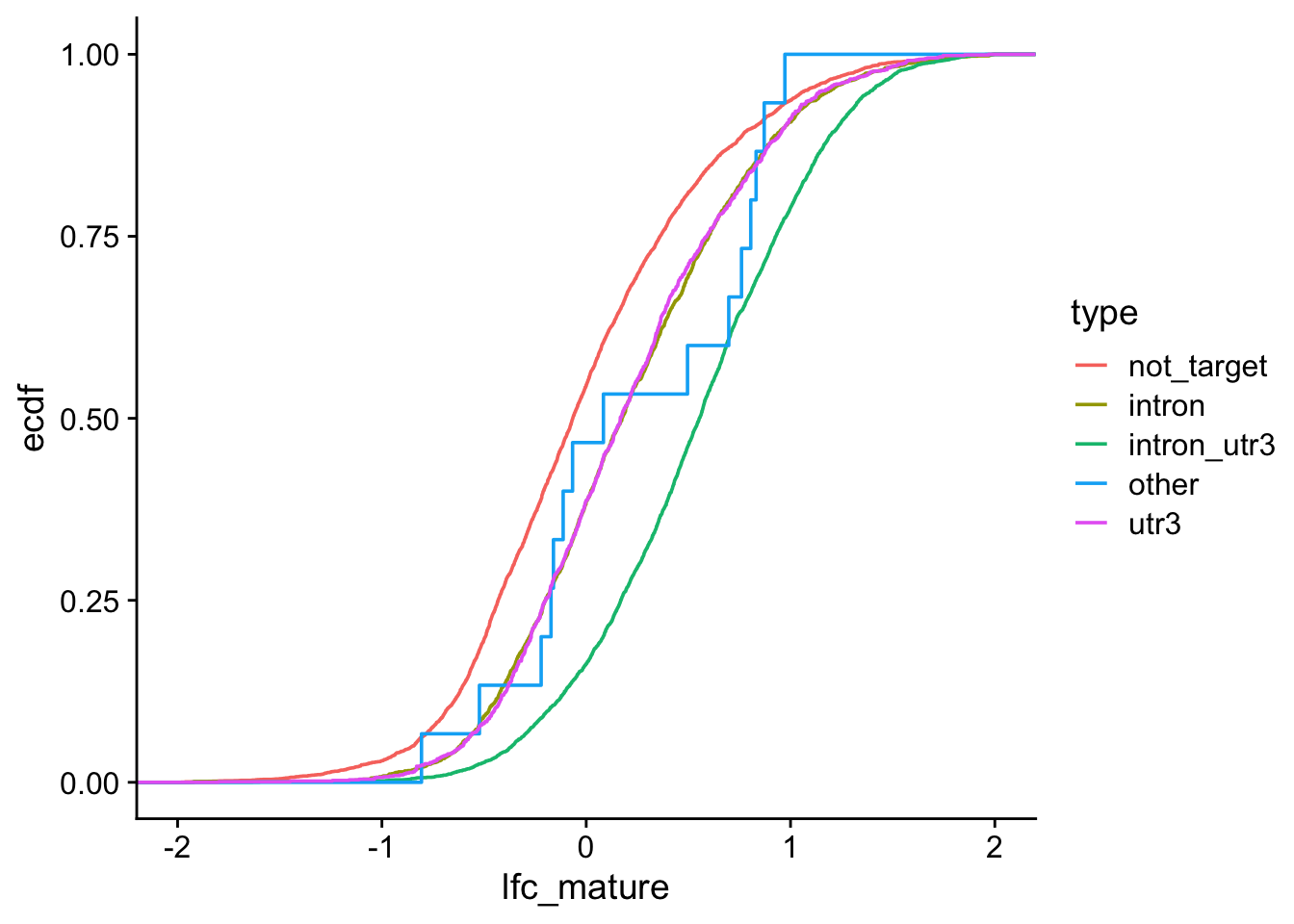
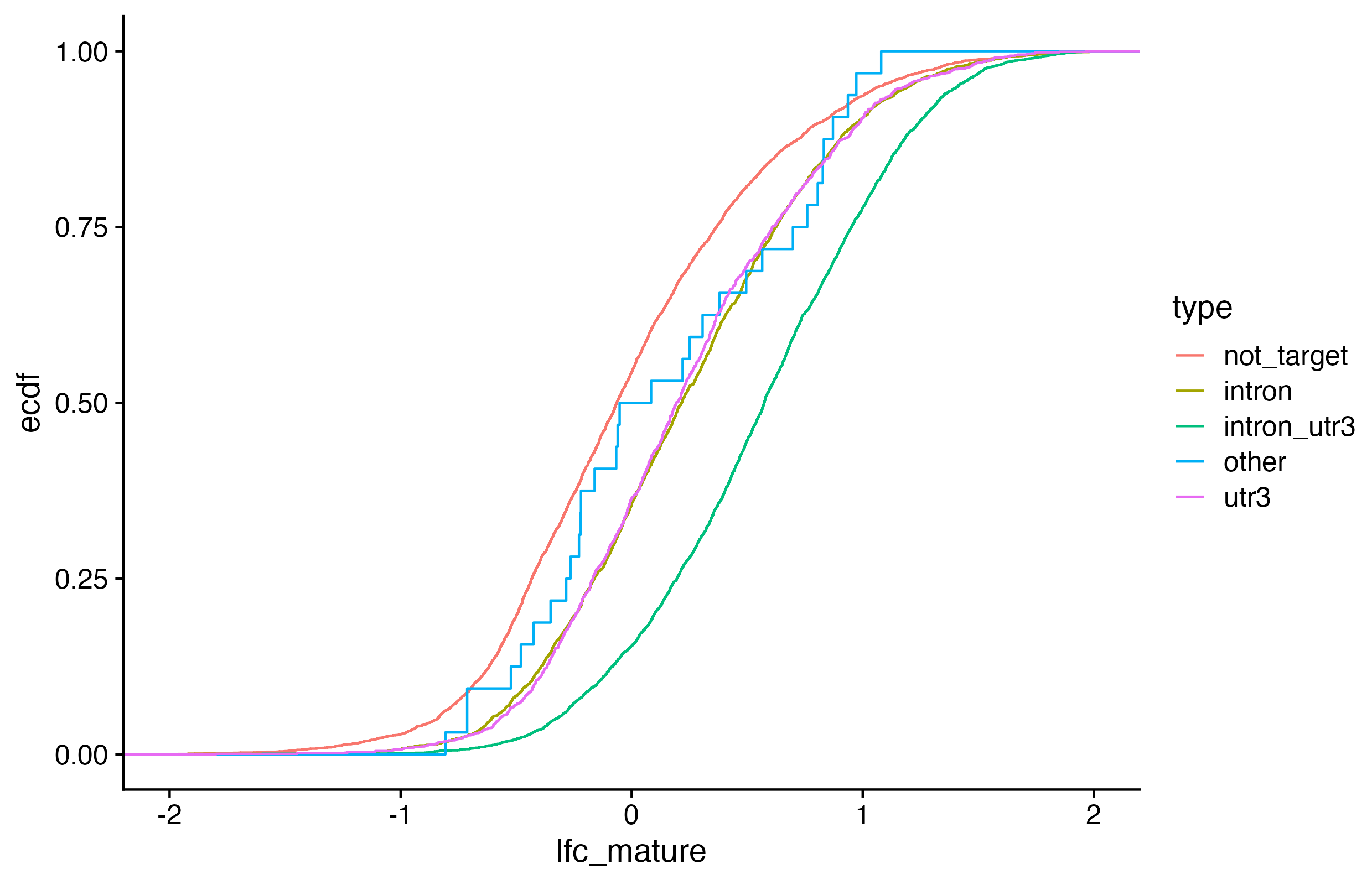
1d. Visualize binding region types and LFC
ggplot(kd_clip, aes(lfc_mature, color =type))+stat_ecdf()+xlim(-2, 2)+theme_cowplot()
Warning: Removed 247 rows containing non-finite outside the scale range
(`stat_ecdf()`).
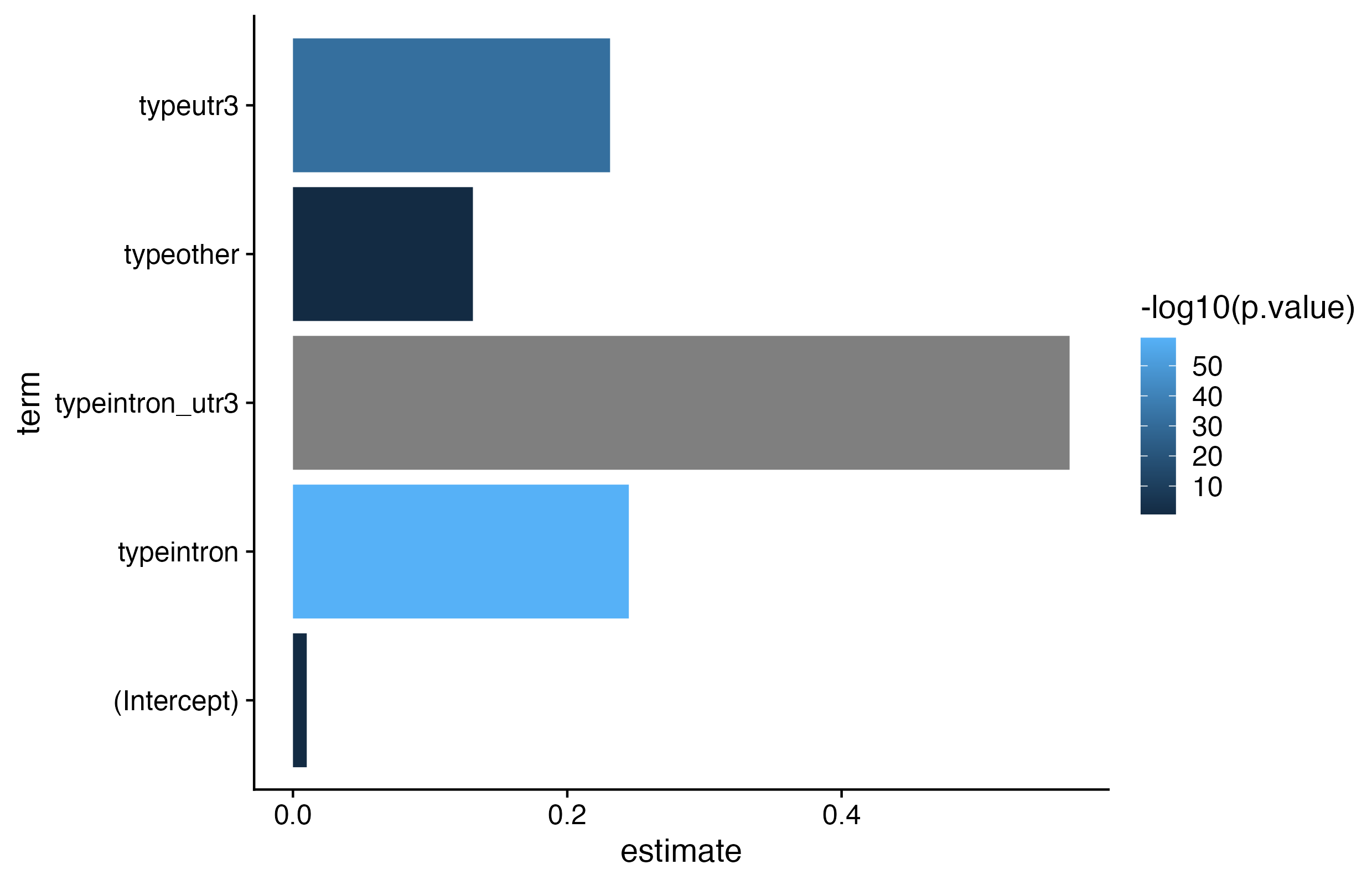
2. Statistical test
Is there a statistically significant different in LFC for the different binding region categories compared to non-targeted RNAs.
# keep only finite values for lfc_mature and lfc_primarykd_clip<-kd_clip[is.finite(kd_clip$lfc_mature), ]# calculate fit using `lm`fit_bins<-lm( data =kd_clip, formula =lfc_mature~type)# examine estimates and p-valsp<-tidy(fit_bins)%>%ggplot( data =.,aes( x =term, y =estimate, fill =-log10(p.value)))+geom_bar(stat ="identity")+coord_flip()+# geom_hline(# yintercept = ref_mean,# color = "red"# ) +theme_cowplot()