RNA Block - Problem Set 28

library(BSgenome.Hsapiens.UCSC.hg19)

Loading required package: BSgenome

Loading required package: BiocGenerics

Loading required package: generics

Attaching package: 'generics'

The following objects are masked from 'package:base':

    as.difftime, as.factor, as.ordered, intersect, is.element, setdiff,
    setequal, union

Attaching package: 'BiocGenerics'

The following objects are masked from 'package:stats':

    IQR, mad, sd, var, xtabs

The following objects are masked from 'package:base':

    anyDuplicated, aperm, append, as.data.frame, basename, cbind,
    colnames, dirname, do.call, duplicated, eval, evalq, Filter, Find,
    get, grep, grepl, is.unsorted, lapply, Map, mapply, match, mget,
    order, paste, pmax, pmax.int, pmin, pmin.int, Position, rank,
    rbind, Reduce, rownames, sapply, saveRDS, table, tapply, unique,
    unsplit, which.max, which.min

Loading required package: S4Vectors

Loading required package: stats4

Attaching package: 'S4Vectors'

The following object is masked from 'package:utils':

    findMatches

The following objects are masked from 'package:base':

    expand.grid, I, unname

Loading required package: IRanges

Loading required package: Seqinfo

Loading required package: GenomicRanges

Loading required package: Biostrings

Loading required package: XVector

Attaching package: 'Biostrings'

The following object is masked from 'package:base':

    strsplit

Loading required package: BiocIO

Loading required package: rtracklayer

library(TxDb.Hsapiens.UCSC.hg19.knownGene)

Loading required package: GenomicFeatures

Loading required package: AnnotationDbi

Loading required package: Biobase

Welcome to Bioconductor

    Vignettes contain introductory material; view with
    'browseVignettes()'. To cite Bioconductor, see
    'citation("Biobase")', and for packages 'citation("pkgname")'.

library(annotatr)
library(org.Hs.eg.db)

library(ggrepel)

Loading required package: ggplot2

library(tidyverse)

── Attaching core tidyverse packages ──────────────────────── tidyverse 2.0.0 ──
✔ dplyr     1.2.0     ✔ readr     2.2.0
✔ forcats   1.0.1     ✔ stringr   1.6.0
✔ lubridate 1.9.5     ✔ tibble    3.3.1
✔ purrr     1.2.1     ✔ tidyr     1.3.2

── Conflicts ────────────────────────────────────────── tidyverse_conflicts() ──
✖ lubridate::%within%() masks IRanges::%within%()
✖ dplyr::collapse()     masks Biostrings::collapse(), IRanges::collapse()
✖ dplyr::combine()      masks Biobase::combine(), BiocGenerics::combine()
✖ purrr::compact()      masks XVector::compact()
✖ dplyr::desc()         masks IRanges::desc()
✖ tidyr::expand()       masks S4Vectors::expand()
✖ dplyr::filter()       masks stats::filter()
✖ dplyr::first()        masks S4Vectors::first()
✖ dplyr::lag()          masks stats::lag()
✖ ggplot2::Position()   masks BiocGenerics::Position(), base::Position()
✖ purrr::reduce()       masks GenomicRanges::reduce(), IRanges::reduce()
✖ dplyr::rename()       masks S4Vectors::rename()
✖ lubridate::second()   masks S4Vectors::second()
✖ lubridate::second<-() masks S4Vectors::second<-()
✖ dplyr::select()       masks AnnotationDbi::select()
✖ dplyr::slice()        masks XVector::slice(), IRanges::slice()
ℹ Use the conflicted package (<http://conflicted.r-lib.org/>) to force all conflicts to become errors

library(cowplot)

Attaching package: 'cowplot'

The following object is masked from 'package:lubridate':

    stamp

library(scales)

Attaching package: 'scales'

The following object is masked from 'package:purrr':

    discard

The following object is masked from 'package:readr':

    col_factor

library(gt)

Attaching package: 'gt'

The following object is masked from 'package:cowplot':

    as_gtable

library(here)

here() starts at /Users/mtaliaferro/Documents/GitHub/molb-7950

Problem Set

Total points: 20. Q1 - 10 pts, Q2 - 10 points each.

Exercises: 1. Identify the transcript regions most enriched for binding by the RBP ZFP36. 2. Within that preferentially bound region, identify which 5mers ZFP36 most likes to bind to.

Remember all the data is available here: rag-tag ENCODE

We are looking for an ZFP36 PAR-CLIP corresponding to this SRA (short-read archive) ID: SRR1046759

1. Determine the annotation region most enriched for ZFP36 binding sites.

To do so you will need to annotate the ZFP36 binding sites and a randomized set of binding sites (based on ZFP36 binding sites) to determine the which binding region is preferred by ZFP36 binding.

1a. Build annotation database

# What annotation categories are available?
possible_annotations <- builtin_annotations()

# Keep only those containing "hg19"
hg19_annots <- grep("hg19_genes", possible_annotations, value = T)


# let's keep 5' utr, cds, intron, 3' utr and intergenic
my_hg19_annots <- hg19_annots[c(3, 4, 7, 10, 11)]


# build the annotation database
annotations <- build_annotations(genome = "hg19", annotations = my_hg19_annots)

'select()' returned 1:1 mapping between keys and columns

Building promoters...

Building 1to5kb upstream of TSS...

Building intergenic...

Building cds...

Building 5UTRs...

Building 3UTRs...

Building exons...

Building introns...

1b. Annotate the ZFP36 binding sites

# We are importing a bed file directly from github for zfp36 binding sites
zfp36_regions <- read_regions(
  con = "https://raw.githubusercontent.com/BIMSBbioinfo/RCAS_meta-analysis/master/rbp-binding-sites/SRR1046759.clusters.bed",
  genome = "hg19", format = "bed"
)


# annotate zfp36 binding sites and convert to df
zfp36_annot <-
  annotate_regions(
    regions = zfp36_regions,
    annotations = annotations,
    ignore.strand = FALSE,
    quiet = FALSE
  ) %>%
  data.frame()

Annotating...

# We will keep only columns we need and collapse the redundant info
myInfo <- c("seqnames", "start", "end", "width", "strand", "annot.symbol", "annot.type")

zfp36_annot <- zfp36_annot[, myInfo] %>%
  unique()

# Just getting rid of the "hg19_genes_" string to simplify `annot.type`
zfp36_annot$annot.type <- gsub("hg19_genes_", "", zfp36_annot$annot.type)

table(zfp36_annot$annot.type)

     3UTRs      5UTRs        cds intergenic    introns 
      1491         19         46        122        885 

1c. Annotate the randomized binding sites

random_regions <- randomize_regions(regions = zfp36_regions, allow.overlaps = TRUE, per.chromosome = TRUE)

Randomizing regions...

random_annot <- annotate_regions(
  regions = random_regions,
  annotations = annotations,
  ignore.strand = FALSE,
  quiet = FALSE
) %>%
  data.frame()

Annotating...

random_annot <- random_annot[, myInfo] %>%
  unique()

random_annot$annot.type <- gsub("hg19_genes_", "", random_annot$annot.type)

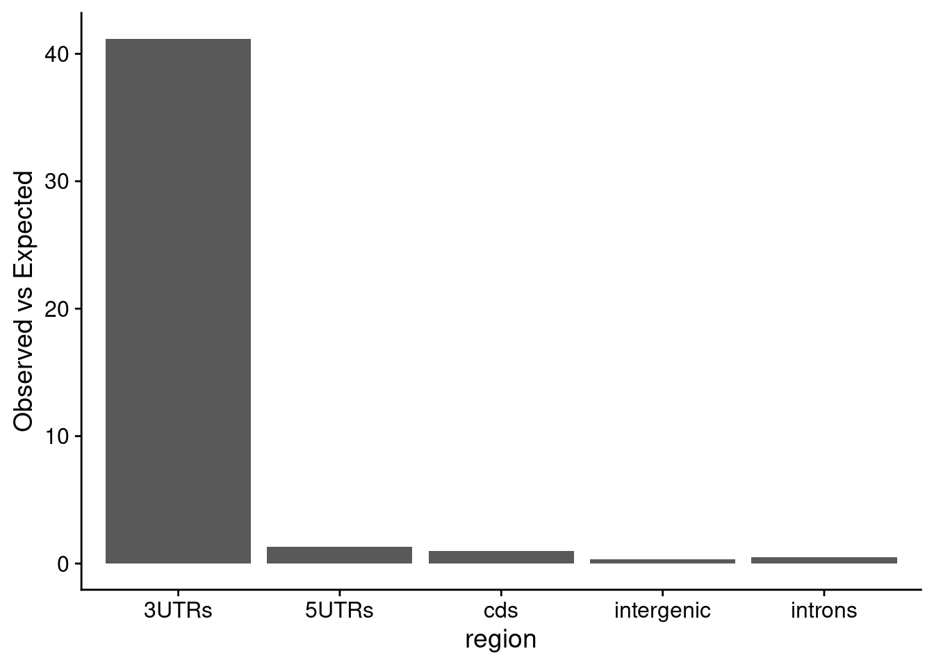
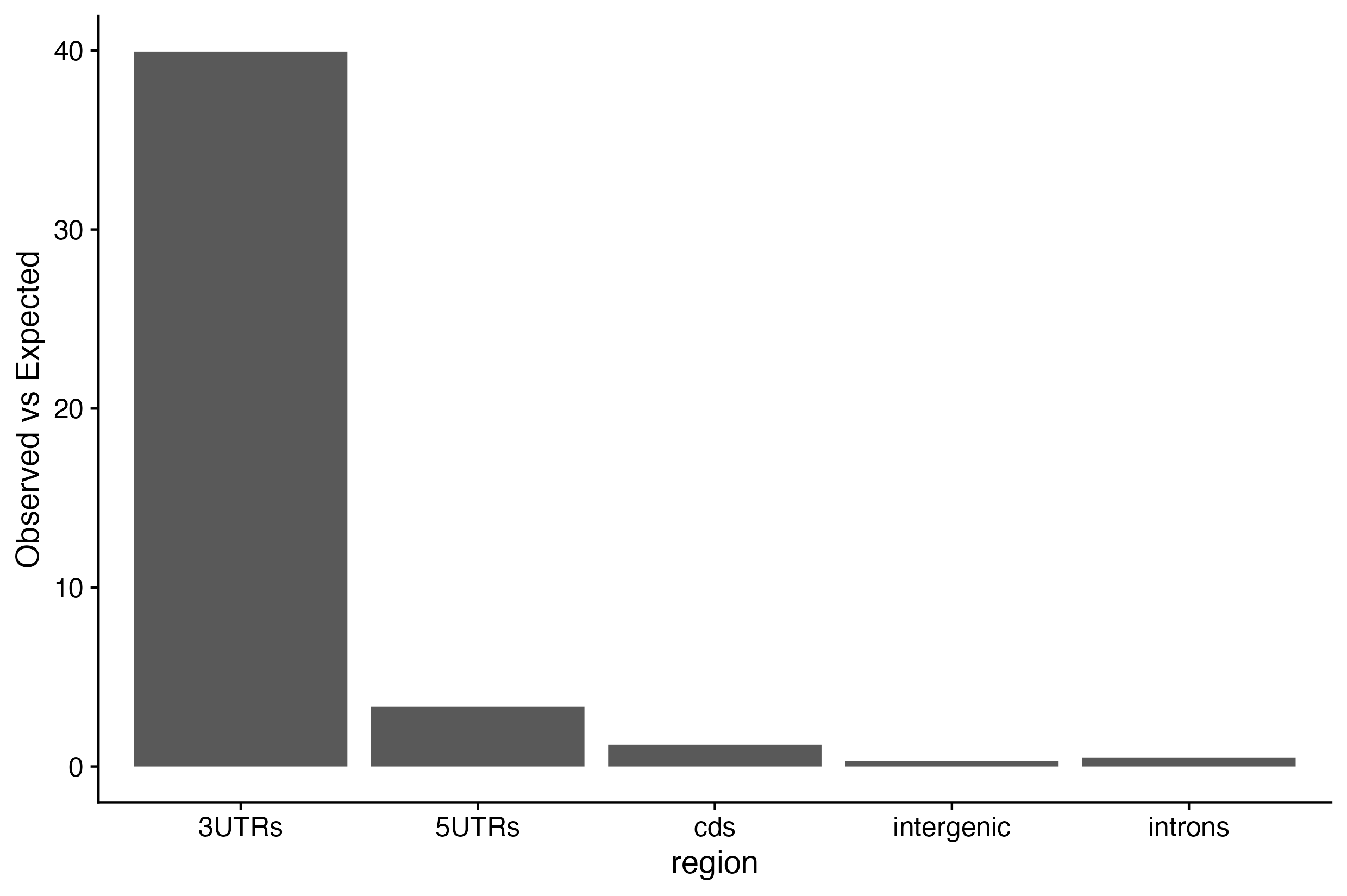
1d. Determine which regions exhibit more than expected ZFP36 binding sites.

site_dist <- bind_cols(
  region = names(table(zfp36_annot$annot.type)),
  observed = table(zfp36_annot$annot.type),
  expected = table(random_annot$annot.type)
)

site_dist$enrichment <- site_dist$observed / site_dist$expected


site_dist_long <- pivot_longer(site_dist, cols = c(observed, expected, enrichment))
colnames(site_dist_long) <- c("region", "type", "value")

ggplot(site_dist_long %>% filter(type == "enrichment"), aes(y = value, x = region)) +
  geom_bar(stat = "identity") +
  ylab("Observed vs Expected") +
  theme_cowplot()

Don't know how to automatically pick scale for object of type <table>.
Defaulting to continuous.

2. Determine the preferred seqeunces bound by ZFP36.

You have determined which region ZFP36 binding sites are preferred to reside - the 3’ UTR :).
Focusing on 3’ UTR binding sites, determine which sequences ZFP36 binds to compared to background sequences for that region USING 5mers.

Remember the workflow for determine k-mer composition (USING 5mers) for any set of intervals (binding sites or annotation categories).

1. Create a Granges object for a given annotation category.
   
2. Remove duplicated intervals (from diff transcript ids) with reduce.
   
3. Retrieve seqeunces using getSeqs
4. Create a dataframe containing the count and frequency of each 5mer.

---

2a. Calculate 5mers in ZFP36 binding sites in 3’ UTRs.

# create a Grange for 3' UTRs

zfp36_3utr <- makeGRangesFromDataFrame(df = zfp36_annot %>% filter(annot.type == "3UTRs"), ignore.strand = F, seqnames.field = "seqnames", start.field = "start", end.field = "end", strand.field = "strand", keep.extra.columns = T)


# get sequencees for those coordinates
zfp36_3utr_seqs <- getSeq(BSgenome.Hsapiens.UCSC.hg19, zfp36_3utr)

# count  all 5mer instances per sequence, add all instances, and turn into a dataframe with column name counts

zfp36_3utr_5mer <- oligonucleotideFrequency(x = zfp36_3utr_seqs, width = 5, as.prob = F, simplify.as = "matrix") %>%
  colSums(.) %>%
  as.data.frame()

colnames(zfp36_3utr_5mer) <- "zfp36_utr_count"

zfp36_3utr_5mer$zfp36_utr_freq <- zfp36_3utr_5mer$zfp36_utr_count / sum(zfp36_3utr_5mer$zfp36_utr_count)

2b. Calculate 5mers in 3’ UTRs.

# create a Grange for 3' UTRs
threeUTR <- GenomicRanges::reduce(annotations[annotations$type %in% my_hg19_annots[4]])

# get  sequencees for those coordinates
threeUTR_seqs <- getSeq(BSgenome.Hsapiens.UCSC.hg19, threeUTR)

# count  all 5mer instances per sequence, add all instances, and turn into a dataframe with column name counts
utr3_5mer <- oligonucleotideFrequency(x = threeUTR_seqs, width = 5, as.prob = F, simplify.as = "matrix") %>%
  colSums(.) %>%
  as.data.frame()

colnames(utr3_5mer) <- "utr_count"

utr3_5mer$utr_freq <- utr3_5mer$utr_count / sum(utr3_5mer$utr_count)

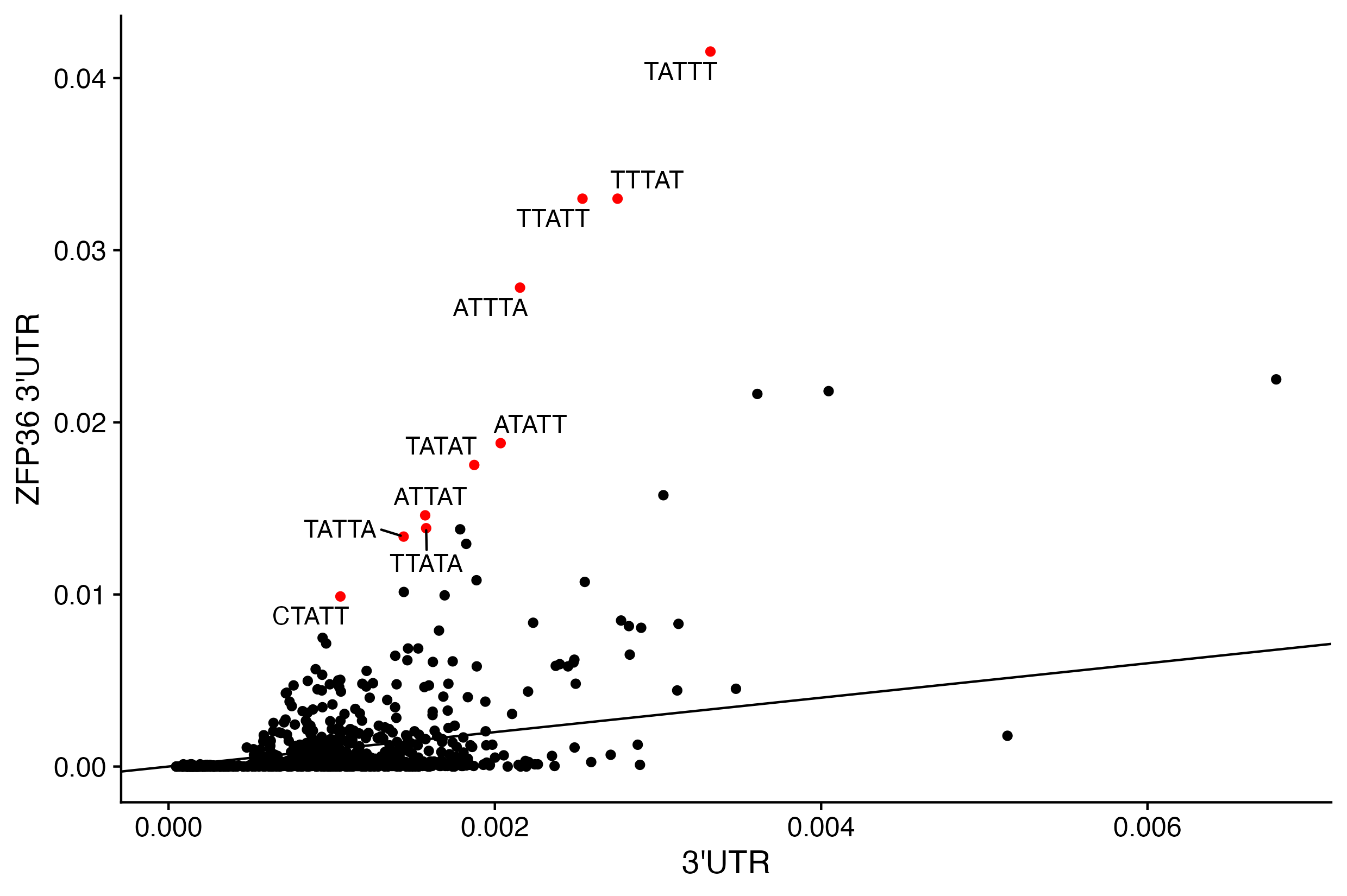
2c. Compare 5mer frequencies in ZFP36 binding sites vs background.

Label 5mers that are 8x, remember log2(8) = 3, enriched above background.

# check if rownames are identical and stop if they are  not
stopifnot(identical(rownames(zfp36_3utr_5mer), rownames(utr3_5mer)))

utr3_df <- bind_cols(zfp36_3utr_5mer, utr3_5mer)

utr3_df$zfp36_enrich <- utr3_df$zfp36_utr_freq / utr3_df$utr_freq


# scatter plot
p_scat <- ggplot(data = utr3_df, aes(y = zfp36_utr_freq, x = utr_freq)) +
  geom_point(color = ifelse(utr3_df$zfp36_enrich > 8, "red", "black")) +
  ylab("ZFP36 3'UTR") +
  xlab("3'UTR") +
  geom_abline(intercept = 0, slope = 1) +
  geom_text_repel(aes(label = ifelse(zfp36_enrich > 8,
    rownames(utr3_df),
    ""
  ))) +
  theme_cowplot()

# print top 10
utr3_df %>%
  rownames_to_column(var = "5mer") %>%
  arrange(-zfp36_enrich) %>%
  top_n(n = 10) %>%
  gt()

Selecting by zfp36_enrich

5mer	zfp36_utr_count	zfp36_utr_freq	utr_count	utr_freq	zfp36_enrich
TTATT	1113	0.032932891	118697	0.002329202	14.139130
ATTTA	932	0.027577228	101781	0.001997258	13.807545
TATTT	1388	0.041069949	153415	0.003010477	13.642341
TTTAT	1090	0.032252338	128213	0.002515936	12.819223
TATAT	593	0.017546455	89168	0.001749752	10.027968
ATATT	628	0.018582081	97312	0.001909562	9.731068
ATTAT	494	0.014617114	77292	0.001516708	9.637395
TATTA	440	0.013019292	68950	0.001353012	9.622450
CTATT	328	0.009705291	51697	0.001014455	9.567000
TTATA	451	0.013344775	74764	0.001467101	9.096017