Problem Set Stats Bootcamp - class 15

Dealing with big data

── Attaching core tidyverse packages ──────────────────────── tidyverse 2.0.0 ──
✔ dplyr     1.1.4     ✔ readr     2.1.5
✔ forcats   1.0.0     ✔ stringr   1.5.1
✔ ggplot2   3.5.2     ✔ tibble    3.3.0
✔ lubridate 1.9.4     ✔ tidyr     1.3.1
✔ purrr     1.1.0     
── Conflicts ────────────────────────────────────────── tidyverse_conflicts() ──
✖ dplyr::filter() masks stats::filter()
✖ dplyr::lag()    masks stats::lag()
ℹ Use the conflicted package (<http://conflicted.r-lib.org/>) to force all conflicts to become errors

Attaching package: 'rstatix'


The following object is masked from 'package:stats':

    filter



Attaching package: 'janitor'


The following object is masked from 'package:rstatix':

    make_clean_names


The following objects are masked from 'package:stats':

    chisq.test, fisher.test


here() starts at /home/runner/work/molb-7950/molb-7950


Attaching package: 'cowplot'


The following object is masked from 'package:lubridate':

    stamp

ang <- read_csv(here("data/bootcamp/edger.csv.gz")) |>
  clean_names() |>
  filter(fdr < 0.05) |>
  select(log_fc_time0_25:log_fc_time8) |>
  as.matrix()

Rows: 17942 Columns: 17
── Column specification ────────────────────────────────────────────────────────
Delimiter: ","
chr  (1): gene
dbl (16): FDR, maxabsfc, logFC.Time0.25, logFC.Time0.5, logFC.Time0.75, logF...

ℹ Use `spec()` to retrieve the full column specification for this data.
ℹ Specify the column types or set `show_col_types = FALSE` to quiet this message.

colnames(ang) <- gsub(pattern = "log_fc_", "", colnames(ang))

Problem # 1

Make sure to run the chunk above. The data represent the avg fold change in gene expression for an angiotensin II time course (.25, .5, .75, 1, 1.5, 2, 3, 4, 6, 8, 24 hrs) compared to unstimulated.

correlation — (7 pts)

Create hierarchical clustering heatmap of pairwise pearson correlation coefficients. And provide 1-2 observations.

#  scale ang (remember the transpose trick)
ang <- t(scale(t(ang)))

# pairwise pearson correlation
p_ang <- cor(ang, method = "pearson")

# make heatmap
pheatmap(
  mat = p_ang,
  clustering_distance_rows = "euclidean",
  clustering_distance_cols = "euclidean",
  clustering_method = "ward.D2"
)

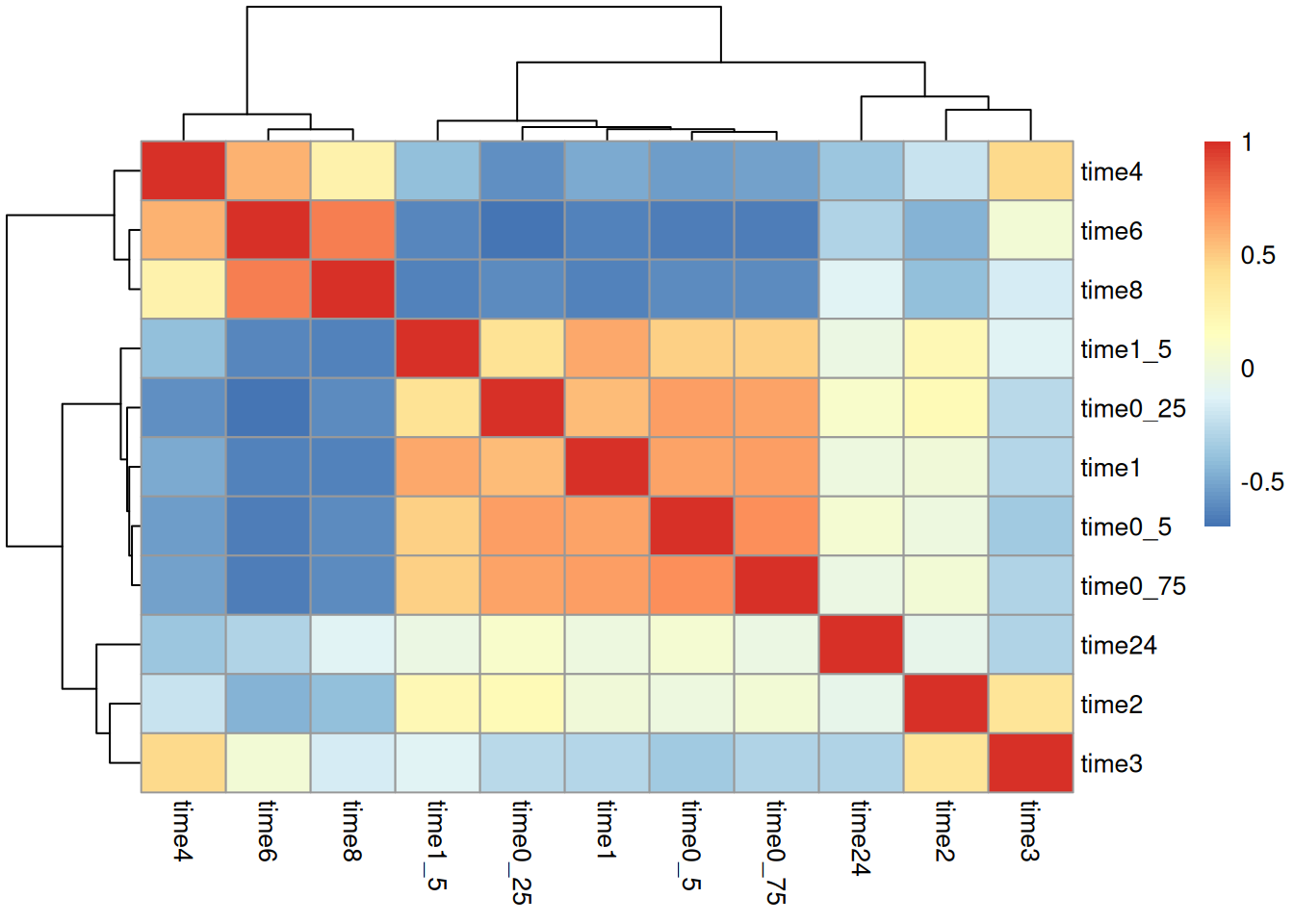
Timepoints close to each other tend to correlate strongly with each other. The 4,6, and 8 hr time points are the most different from all others.

PCA — (7 pts)

Perform PCA and visualize PC1 vs PC2.Provide 1-2 observations.

pc_ang <- prcomp(ang)

# gather info from summary
pca_data_info <- summary(pc_ang)$importance |> as.data.frame()

pca_data_info <- round(x = pca_data_info, digits = 3)

# we make a dataframe out of the rotations and will use this to plot
pca_plot_data <- pc_ang$rotation |>
  as.data.frame() |>
  rownames_to_column(var = "ID")

# plot
ggplot(data = pca_plot_data, mapping = aes(x = PC1, y = PC2, color = ID)) +
  geom_point(size = 3) +
  labs(
    x = paste("PC1, %", 100 * pca_data_info["Proportion of Variance", "PC1"]),
    y = paste("PC2, %", 100 * pca_data_info["Proportion of Variance", "PC2"]),
    title = "PCA for angII timecourse"
  ) +
  theme_cowplot()

There is a a circular patter that seems to correspond to the timepoints. Interestingly, 24 appears to group back with 0.25 indicating the system is resetting w/respect to RNA levels.

Calculate the empirical p-value of the cluster most enriched for DUX4 targets by sampling — (6 pts)

step 1:

• identify which cluster is the most enriched for DUX4 targets using Geneoverlap.
• assign the cluster number as a variable named c to use later.

# read in data
cd <- read_tsv(here("data", "dux4_clustering_results.csv.gz"))

# list of genes by dux4 targeting
duxList <- split(cd$gene_symbol, cd$target)

# list of genes by clustering
clustList <- split(cd$gene_symbol, as.factor(cd$Cluster))

# calculate all overlaps between lists
gom.duxclust <- newGOM(duxList,
                       clustList,
                       genome.size = nrow(cd)
                       )

# retrieve p-values for each cluster and sort
getMatrix(gom.duxclust, "pval") |>
  t() |>
  as.data.frame() |>
  rownames_to_column(var = "clust") |>
  as.tibble() |>
  arrange(target)

# which cluster has the lowest p-value?
c <- 5

step 2:

• determine the number of total genes in that cluster. save this as a variable named cN to use later. you will need to know this to figure out how many genes to sample from the whole data set. the size matching will make it so the random samples in your null distribution is better matched to your observation specific to the cluster of interest.

• determine the number of DUX4 targets in the cluster. save this as a variable named cNt to use later. this is the number that you are interested in comparing between the null distribution and your observation. remember, the p-value tells you the probability that the null hypothesis could generate an equal or more extreme observation.

# how many genes are in cluster 5?
cN <- cd |>
  filter(Cluster == "5") |>
  nrow()

# how many dux targets are in cluster 5?
cNt <- cd |>
  filter(Cluster == "5" & target == "target") |>
  nrow()

step 3:

generate 1000 random sample of the size cN from all genes in the data set, and for each random sample save the number of genes that are DUX4 targets. this is your null distribution.

visualize the distribution of the # of DUX4 targets in these 1000 random (your null distribution) and overlay the number of DUX4 targets you observed in the cluster that was most enriched for DUX4 targets, cNt.

# first simplify the problem by figuring out the # of DUX4 targets for 1 random sample
sample_n(tbl = cd, size = cN) |>
  filter(target == "target") |>
  nrow()
  

# create an empty vector for storing the # dux targets for each iteration. call this `sampled_targets`
sampled_targets <- vector()


# then use a for loop to do it 1000 times and save the results in `sampled_targets`

for (i in 1:1000) {
  sampled_targets[i] <- sample_n(tbl = cd, size = cN) |>
  filter(target == "target") |>
  nrow()
}

ggplot(n, aes(x = sampled_targets)) +
  geom_density() +
  geom_vline(xintercept = cNt, color = "red") +
  theme_cowplot()

# how many times did a simulation have more dux4 targets than `cNt`
sampled_targets[sampled_targets > cNt] |>
  length()

What is the p-value?

p < 0.001

What is your interpretation?

The null hypothesis that the number of DUX4 targets in cluster 5 IS NOT WELL SUPPORTED.

The number of DUX4 targets in c5 is very unlikely to be explained by chance.