Problem Set Stats Bootcamp - class 14

Hypothesis Testing

library(tidyverse)
library(rstatix)
library(ggpubr)
library(gt)
library(janitor)
library(here)
library(cowplot)
library(broom)

biochem <- read_tsv(
  "http://mtweb.cs.ucl.ac.uk/HSMICE/PHENOTYPES/Biochemistry.txt",
  show_col_types = FALSE
) |>
  janitor::clean_names()

# simplify names a bit more
colnames(biochem) <- gsub(
  pattern = "biochem_",
  replacement = "",
  colnames(biochem)
)

# we are going to simplify this a bit and only keep some columns
keep <- colnames(biochem)[c(1, 6, 9, 14, 15, 24:28)]
biochem <- biochem[, keep]

# get weights for each individual mouse
# careful: did not come with column names
weight <- read_tsv(
  "http://mtweb.cs.ucl.ac.uk/HSMICE/PHENOTYPES/weight",
  col_names = F,
  show_col_types = FALSE
)

# add column names
colnames(weight) <- c("subject_name", "weight")

# add weight to biochem table and get rid of NAs
# rename gender to sex
b <- inner_join(biochem, weight, by = "subject_name") |>
  na.omit() |>
  rename(sex = gender)

Problem # 1

Can mouse sex explain mouse cholesterol? {.smaller}

STEP 1: Null hypothesis and variable specification — (2 pts)

\(\mathcal{H}_0:\) mouse \(sex\) does NOT explain \(cholesterol\)

\(cholesterol\) is the response variable

\(sex\) is the explanatory variable

STEP 2: Fit linear model and examine results — (3 pts)

fit_cs <- lm(formula = tot_cholesterol ~ 1 + sex, data = b)

Fit summary:

glance(fit_cs) |>
  gt() |>
  fmt_number(columns = r.squared:statistic, decimals = 3)

r.squared	adj.r.squared	sigma	statistic	p.value	df	logLik	AIC	BIC	deviance	df.residual	nobs
0.184	0.183	0.576	400.774	1.425116e-80	1	-1546.04	3098.081	3114.537	591.5753	1780	1782

Coefficient summary:

tidy(fit_cs) |>
  gt() |>
  fmt_number(columns = estimate:statistic, decimals = 3)

term	estimate	std.error	statistic	p.value
(Intercept)	2.797	0.019	144.812	0.000000e+00
sexM	0.547	0.027	20.019	1.425116e-80

Collecting residuals and other information — (2 pts)

add residuals and other information

# augment
b_cs <- augment(fit_cs, data = b)


avg_c <- mean(b_cs$tot_cholesterol)

c <- b |>
  group_by(sex) |>
  get_summary_stats(tot_cholesterol, type = "mean")


# mean chol female
avg_cf <- pull(c[1, 4])


# mean chol male
avg_cm <- pull(c[2, 4])

STEP 4: Visualize the error around fit — (2 pts)

# plot of data with mean and colored by residuals
p_cs <- ggplot(
  b_cs,
  aes(x = sex, y = tot_cholesterol)
) +
  geom_point(
    position = position_jitter(),
    aes(color = .resid)
  ) +
  scale_color_gradient2(
    low = "blue",
    mid = "black",
    high = "yellow"
  ) +
  geom_hline(
    yintercept = avg_c,
    color = "darkgrey"
  ) +
  geom_segment(
    aes(
      x = .5,
      xend = 1.5,
      y = avg_cf,
      yend = avg_cf
    ),
    color = "red"
  ) +
  geom_segment(
    aes(
      x = 1.5,
      xend = 2.5,
      y = avg_cm
    ),
    yend = avg_cm,
    color = "red"
  ) +
  theme_cowplot()

p_cs

Warning in geom_segment(aes(x = 0.5, xend = 1.5, y = avg_cf, yend = avg_cf), : All aesthetics have length 1, but the data has 1782 rows.
ℹ Please consider using `annotate()` or provide this layer with data containing
  a single row.

Warning in geom_segment(aes(x = 1.5, xend = 2.5, y = avg_cm), yend = avg_cm, : All aesthetics have length 1, but the data has 1782 rows.
ℹ Please consider using `annotate()` or provide this layer with data containing
  a single row.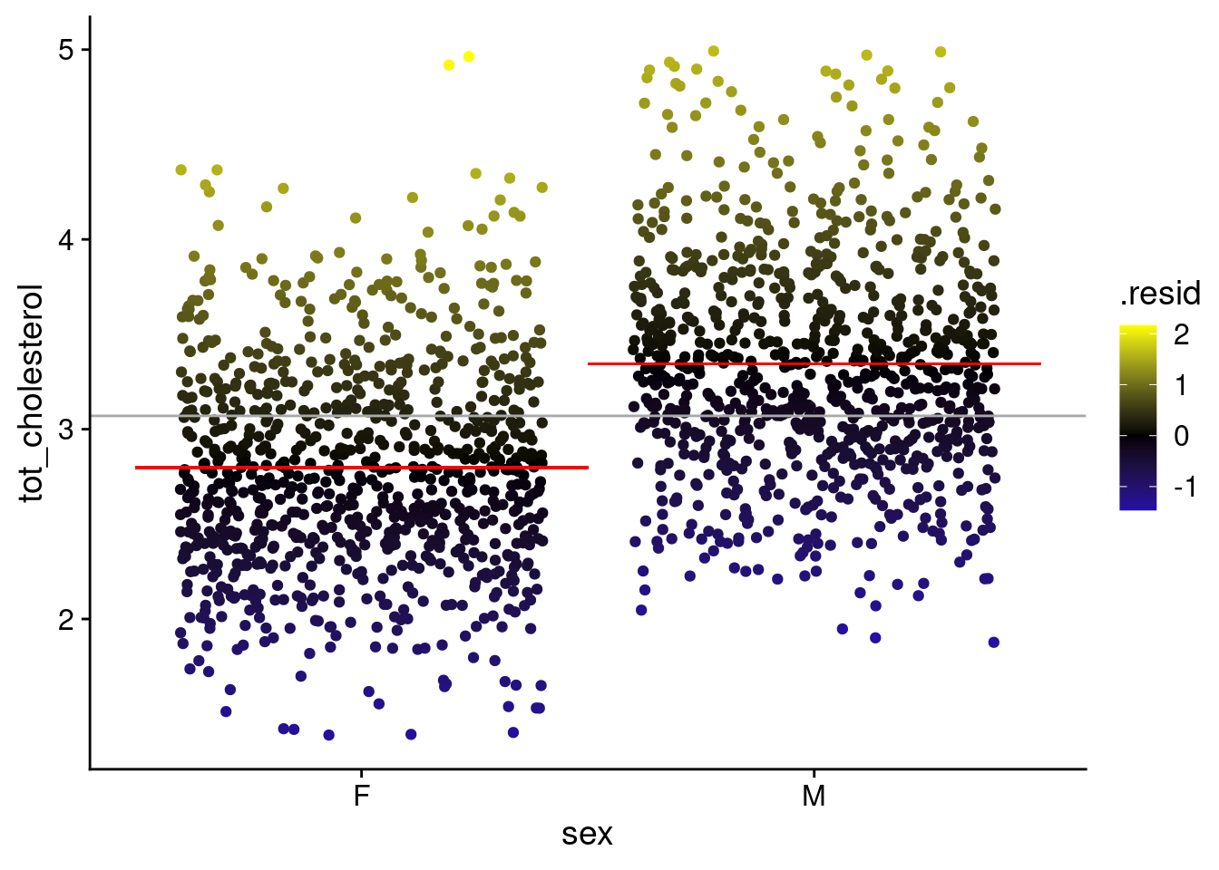

STEP 5: Visualize the error around the null (mean weight) — (2 pts)

p_c <- ggplot(
  b_cs,
  aes(x = sex, y = tot_cholesterol)
) +
  geom_point(
    position = position_jitter(),
    aes(color = tot_cholesterol - avg_c)
  ) +
  scale_color_gradient2(
    low = "blue",
    mid = "black",
    high = "yellow"
  ) +
  geom_hline(
    yintercept = avg_c,
    color = "darkgrey"
  ) +
  theme_cowplot()

p_c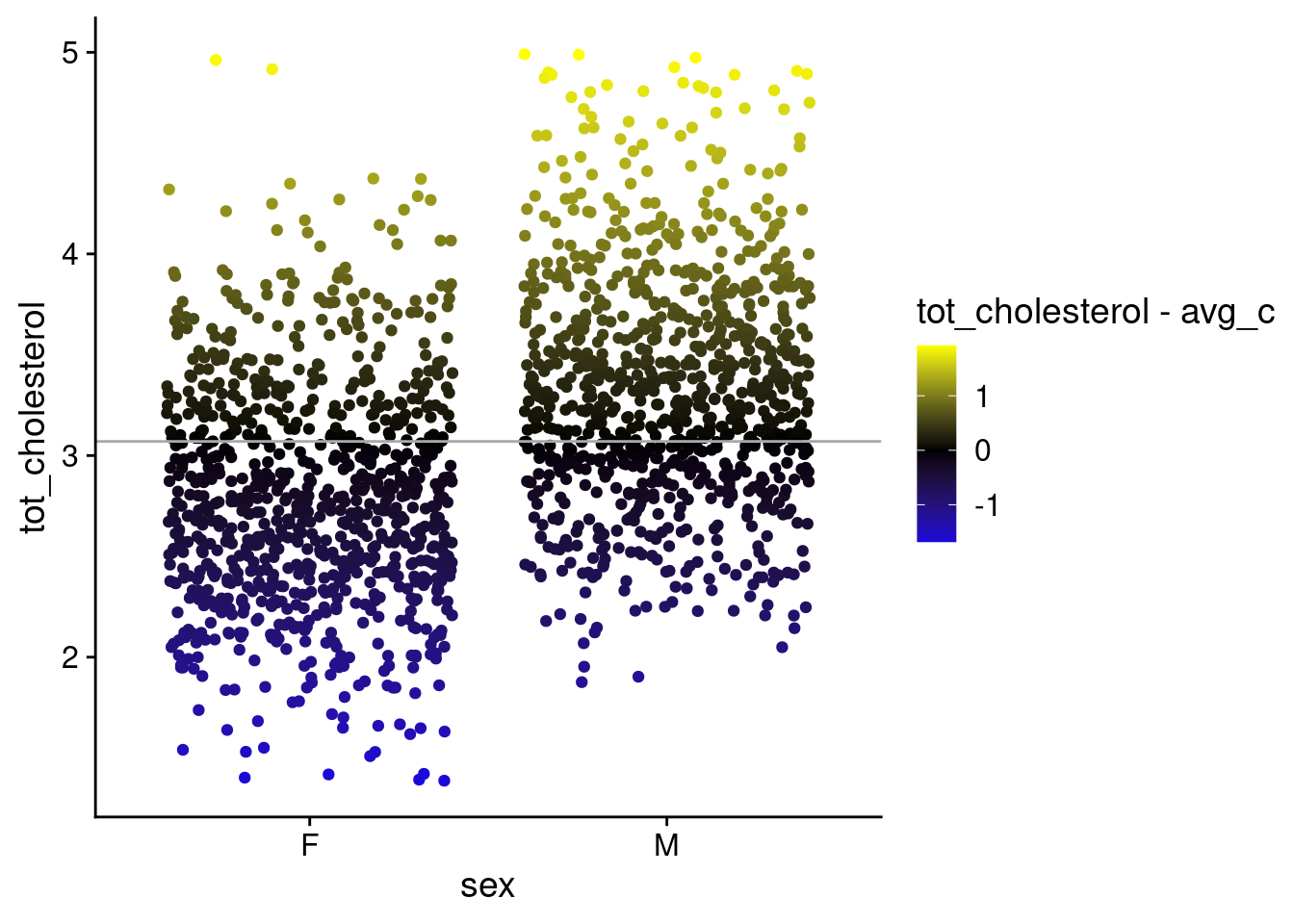

Plot the fit error and the null error as 2 panels — (2 pts)

plot_grid(p_cs, p_c, ncol = 2, labels = c("cholesterol by sex", "cholesterol"))

Warning in geom_segment(aes(x = 0.5, xend = 1.5, y = avg_cf, yend = avg_cf), : All aesthetics have length 1, but the data has 1782 rows.
ℹ Please consider using `annotate()` or provide this layer with data containing
  a single row.

Warning in geom_segment(aes(x = 1.5, xend = 2.5, y = avg_cm), yend = avg_cm, : All aesthetics have length 1, but the data has 1782 rows.
ℹ Please consider using `annotate()` or provide this layer with data containing
  a single row.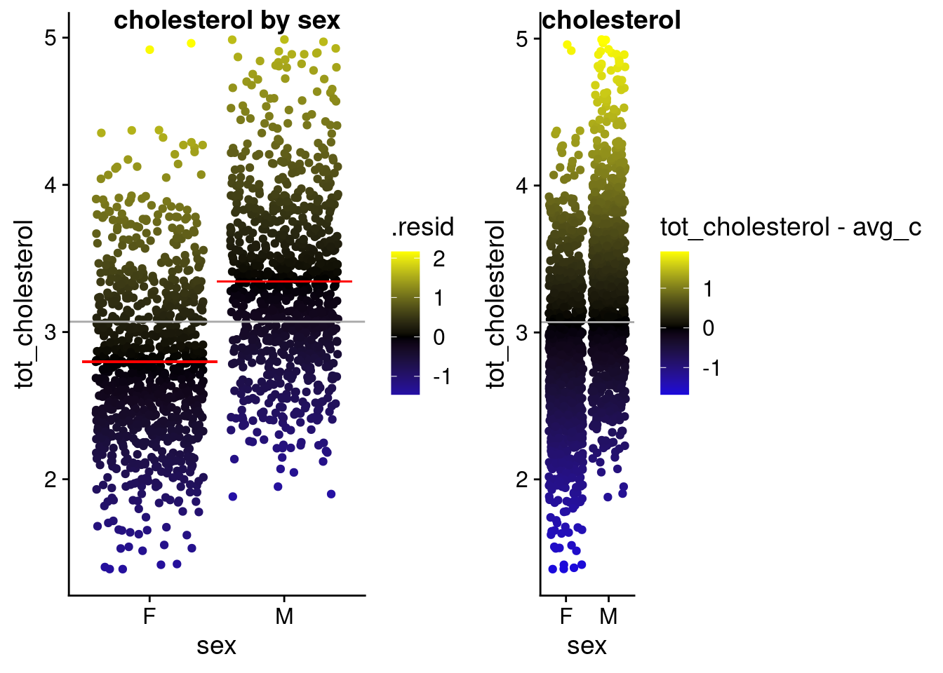

Calculate \(R^2\) — (3 pts)

ss_fit <- sum(b_cs$.resid^2)

ss_null <- sum(
  (b_cs$tot_cholesterol - avg_c)^2
)

\(R^2 = 1 - \displaystyle \frac {SS_{fit}}{SS_{null}}\)

rsq <- 1 - ss_fit / ss_null
rsq

[1] 0.1837759

check agains Rsq in your fit

glance(fit_cs) |> select(r.squared)

# A tibble: 1 × 1
  r.squared
      <dbl>
1     0.184

Compare to traditional t-test — (2 pts)

# run analagous t-test
b |>
  t_test(tot_cholesterol ~ 1 + sex) |>
  select(-c(n1, n2, df)) |>
  gt()

.y.	group1	group2	statistic	p
tot_cholesterol	F	M	-20.01933	1.46e-80

tidy(fit_cs) |>
  select(term, estimate, statistic, p.value) |>
  gt()

term	estimate	statistic	p.value
(Intercept)	2.7968013	144.81230	0.000000e+00
sexM	0.5467901	20.01933	1.425116e-80

Provide your interpretation of the result — (2 pts)

The null model that mouse \(sex\) does NOT explain \(cholesterol\) is not well supported. Therefore, i believe that mouse \(sex\) is able to explain ~%18 of the variation in \(cholesterol\).