Problem Set Stats Bootcamp - class 13

Hypothesis Testing

library(tidyverse)
library(rstatix)
library(ggpubr)
library(gt)
library(janitor)
library(here)
library(broom)

biochem <- read_tsv(
  "http://mtweb.cs.ucl.ac.uk/HSMICE/PHENOTYPES/Biochemistry.txt",
  show_col_types = FALSE
) |>
  janitor::clean_names()

# simplify names a bit more
colnames(biochem) <- gsub(
  pattern = "biochem_",
  replacement = "",
  colnames(biochem)
)

# we are going to simplify this a bit and only keep some columns
keep <- colnames(biochem)[c(1, 6, 9, 14, 15, 24:28)]
biochem <- biochem[, keep]

# get weights for each individual mouse
# careful: did not come with column names
weight <- read_tsv(
  "http://mtweb.cs.ucl.ac.uk/HSMICE/PHENOTYPES/weight",
  col_names = F,
  show_col_types = FALSE
)

# add column names
colnames(weight) <- c("subject_name", "weight")

# add weight to biochem table and get rid of NAs
# rename gender to sex
b <- inner_join(biochem, weight, by = "subject_name") |>
  na.omit() |>
  rename(sex = gender)

Problem # 1

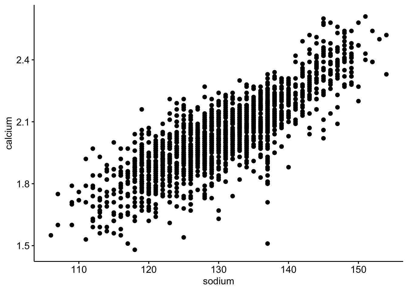
Is there an association between mouse calcium and sodium levels?

1. Make a scatterplot to inspect variable — (2 pts)

ggscatter(
  data = b,
  y = "calcium",
  x = "sodium"
)

2. Are they normal (enough)? — (1 pts)

ggqqplot(data = b, x = "calcium")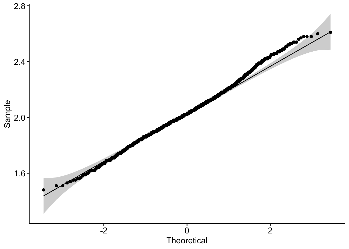

b |> shapiro_test(calcium)

# A tibble: 1 × 3
  variable statistic         p
  <chr>        <dbl>     <dbl>
1 calcium      0.995 0.0000108

ggqqplot(data = b, x = "sodium")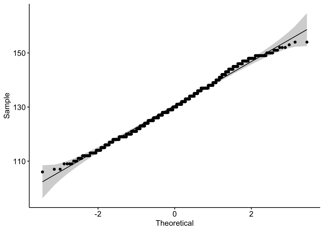

b |> shapiro_test(sodium)

# A tibble: 1 × 3
  variable statistic          p
  <chr>        <dbl>      <dbl>
1 sodium       0.995 0.00000432

Which test will you use and why?

I will use the Pearson since the qqplots look ok and there are ~1700 observations. Spearman is fine too - especially since sodium looks a little like an integer and not continuous.

3. Declare null hypothesis \(\mathcal{H}_0\) — (1 pts)

\(\mathcal{H}_0\) is that there is no dependency/association between \(calcium\) and \(sodium\)

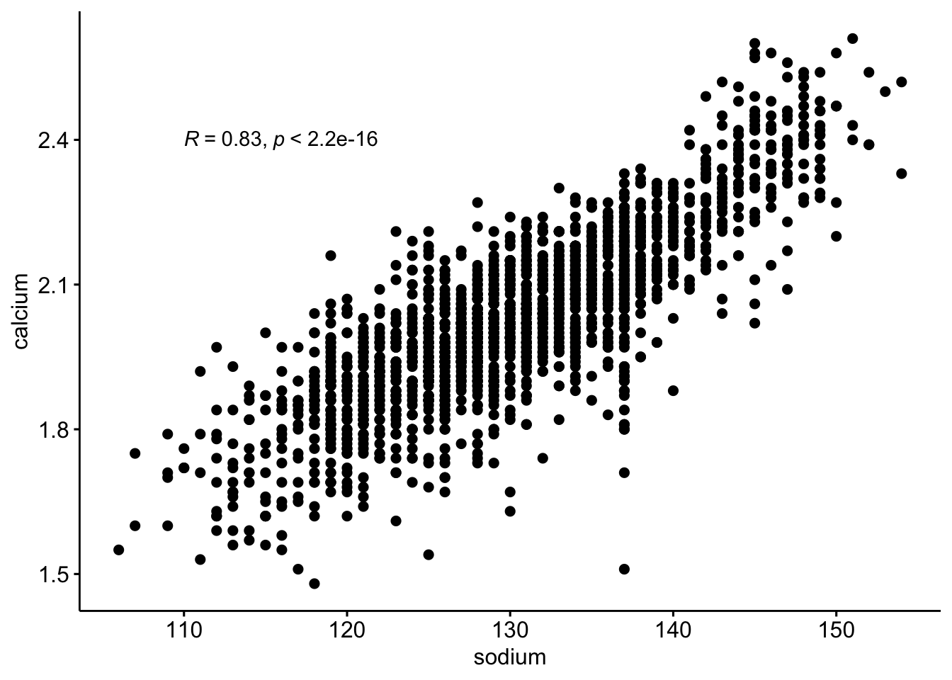
4. Calculate and plot the correlation on a scatterplot — (2 pts)

ggscatter(
  data = b,
  y = "calcium",
  x = "sodium"
) +
  stat_cor(
    method = "pearson",
    label.x = 110,
    label.y = 2.4
  )

Problem # 2

Do mouse calcium levels explain mouse sodium levels? If so, to what extent?

Use a linear model to do the following:

1. Specify the Response and Explanatory variables — (2 pts)

The response variable y is sodium The explantory variable x is calcium

2. Declare the null hypothesis — (1 pts)

The null hypothesis is calcium levels do not explain/predict sodium levels.

3. Use the lm function to create a fit (linear model) — (1 pts)

also save the slope and intercept for later

fit <- lm(formula = sodium ~ 1 + calcium, data = b)


int <- tidy(fit)[1, 2]
slope <- tidy(fit)[2, 2]

4. Add residuals to the data and create a plot visualizing the residuals — (1 pts)

b_fit <- augment(fit, data = b)

avg_sod <- mean(b$sodium)

ggplot(
  data = b_fit,
  aes(x = calcium, y = sodium)
) +
  geom_point(size = 1, aes(color = .resid)) +
  geom_abline(
    intercept = pull(int),
    slope = pull(slope),
    col = "red"
  ) +
  scale_color_gradient2(
    low = "blue",
    mid = "black",
    high = "yellow"
  ) +
  geom_segment(
    aes(
      xend = calcium,
      yend = .fitted
    ),
    alpha = .1
  ) + # plot line representing residuals
  theme_linedraw()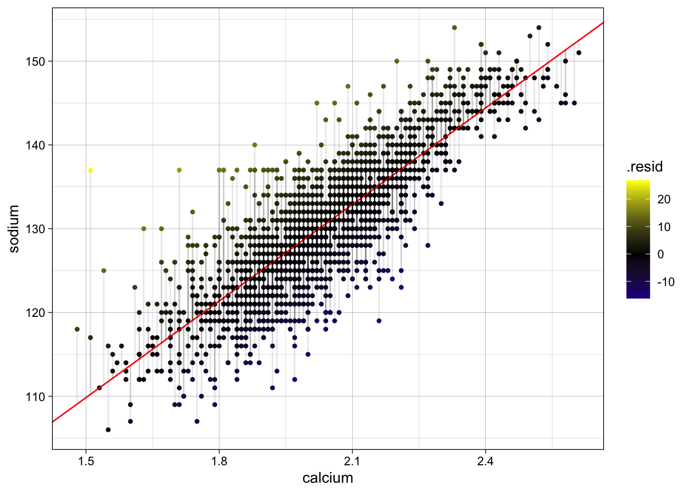

5. Calculate the \(R^2\) and compare to \(R^2\) from fit — (2 pts)

\(R^2 = 1 - \displaystyle \frac {SS_{fit}}{SS_{null}}\)

\(SS_{fit} = \sum_{i=1}^{n} (data - line)^2 = \sum_{i=1}^{n} (y_{i} - (\beta_0 \cdot 1+ \beta_1 \cdot x)^2\)

\(SS_{null}\) — sum of squared errors around the mean of \(y\)

\(SS_{null} = \sum_{i=1}^{n} (data - mean)^2 = \sum_{i=1}^{n} (y_{i} - \overline{y})^2\)

ss_fit <- sum(b_fit$.resid^2)
ss_null <- sum(
  (b_fit$sodium - avg_sod)^2
)
rsq <- 1 - ss_fit / ss_null
glance(fit) |> select(r.squared)

# A tibble: 1 × 1
  r.squared
      <dbl>
1     0.684

6. Using \(R^2\), describe the extent to which calcium explains sodium levels — (2 pts)

\(calcium\) explains ~68% of variation in \(sodium\) levels

7. Report (do not calculate) the \(p-value\) and your decision on the null — (1 pts)

fit |>
  glance() |>
  select(p.value)

# A tibble: 1 × 1
  p.value
    <dbl>
1       0

The null hypothesis is calcium levels do not explain/predict sodium levels IS NOT SUPPORTED

Calcium levels to predict sodium levels.

Problem # 3

What is the association between mouse weight and age levels for different sexes?

1. Calculate the pearson correlation coefficient between weight and age for females and males — (2 pts)

b |>
  group_by(factor(sex)) |>
  cor_test(weight, age)

# A tibble: 2 × 9
  `factor(sex)` var1   var2    cor statistic        p conf.low conf.high method 
  <fct>         <chr>  <chr> <dbl>     <dbl>    <dbl>    <dbl>     <dbl> <chr>  
1 F             weight age    0.21      6.30 4.67e-10    0.143     0.269 Pearson
2 M             weight age    0.37     12.0  1.22e-30    0.314     0.427 Pearson

2. Describe your observations — (2 pts)

The relationship between weight and age is stronger for males than it is for females.