possible_annotations <- builtin_annotations()

# grep to keep those containing "hg19"
hg19_annots <- grep(
  "??_genes",
  possible_annotations,
  value = T)

# WHY DID WE PICK hg19?

# let's keep 5' utr, cds, intron, 3' utr and intergenic
my_hg19_annots <- hg19_annots[c(3,4,7,10,11)]

# build the annotation database
annotations <- build_annotations(
  genome = 'hg19',
  annotations = ??)

annotationsRBP-RNA part 1
Learning Objectives
Describe the steps involved in performing CLIP-seq experiment to identify RBP binding sites transcriptome-wide.
Understand how CLIP-seq data is processed from reads to generate binding sites.
Assign the binding sites to genes and transcipt regions - 3’ UTR, CDS, intron, etc.
Determine the sequences bound by the RBP using proper background sequence models.
Background
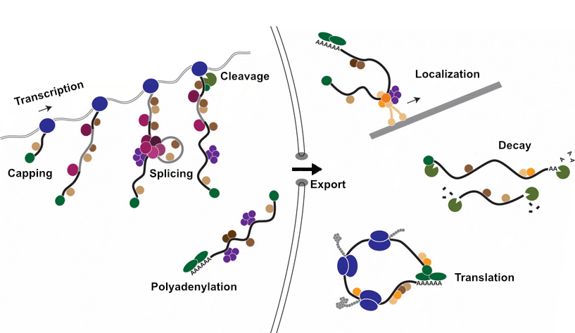
RNA-binding proteins (RBPs) interact with RNAs to control every regulatory step from transcription to translation.
RBPs bind to specific regulatory elements with RNAs. These regulatory elements are specific sequence and/or structures recognized by the RBPs.
For example, an RBP might bind to specific sequences in the 3’ UTR of an mRNA and recruit enzymes to promote deadenylation (removal of polyA tails) and subsequent target RNA decay.
Why do we need to know binding sites?

- RBPs and microRNAs recognize short sequences: 4-7 nucleotides.
- These sequences appear quite frequently (purple) in a 3’ UTR.
- Conservation is often used to focus sites more likely to be functional/important.
- However, the binding evidence allows one to know the functional regulatory element.
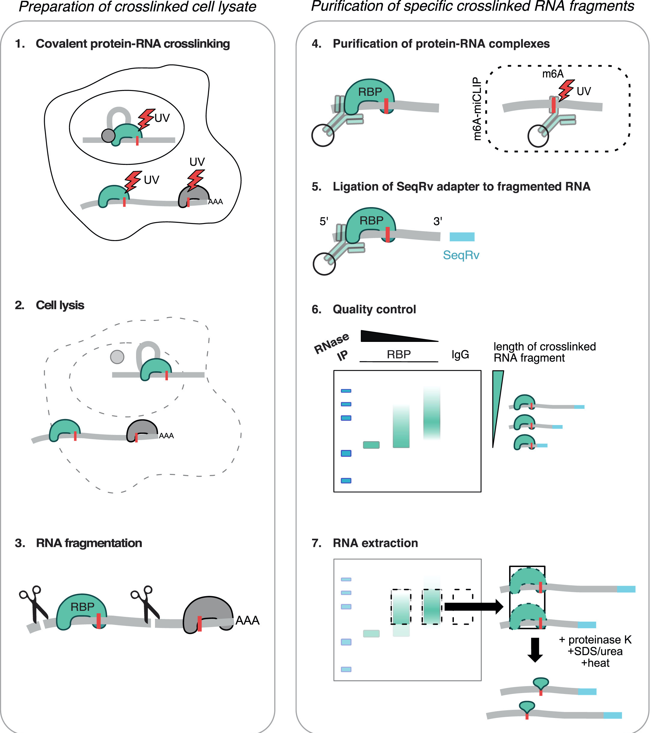
Mapping of RBP binding sites: CLIP-seq
- Covalent cross-linking of RBPs to RNA using 254 nm UV light.
- Lyse cells
- Mild digestion with RNase (leaving protein protected RNA fragments )
- Immunoprecipitate your RBP of interest (better have a good antibody)
- Ligate labeled 3’ adapter RNA
- Cut out region corresponding to crosslinked RBP (and matched input)
- Proteinase K treat and isolate RNA
- Reverse transcription
- Make library from cDNA fragments and SEQUENCE!
Mapping of RBP binding sites: PAR-CLIP
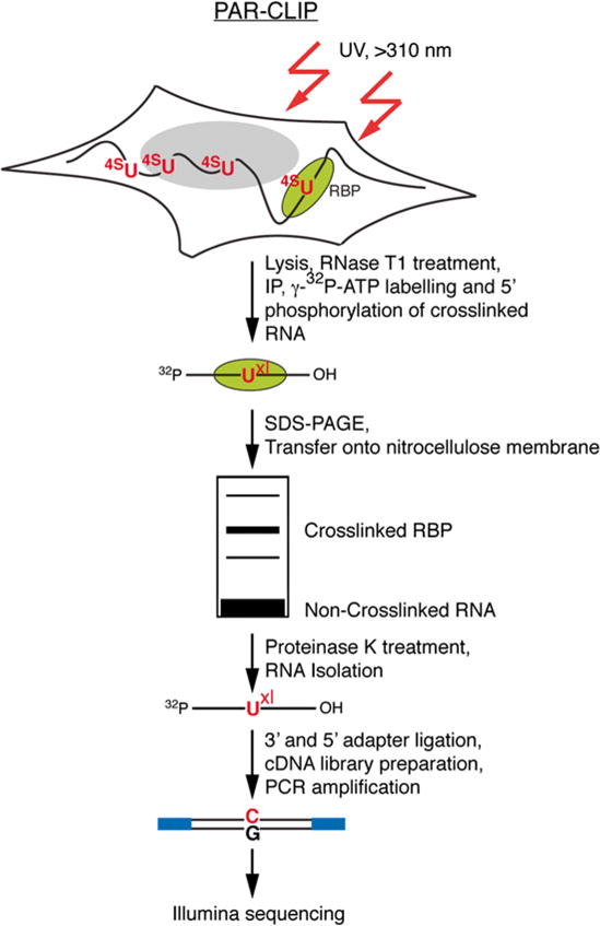
PAR-CLIP: photoactivatable ribonucleoside enhanced clip
- 4-thiouridine (4sU) incorporation increases cross-linking efficiency
- Cross-linking ~310 nm UV (blacklight)
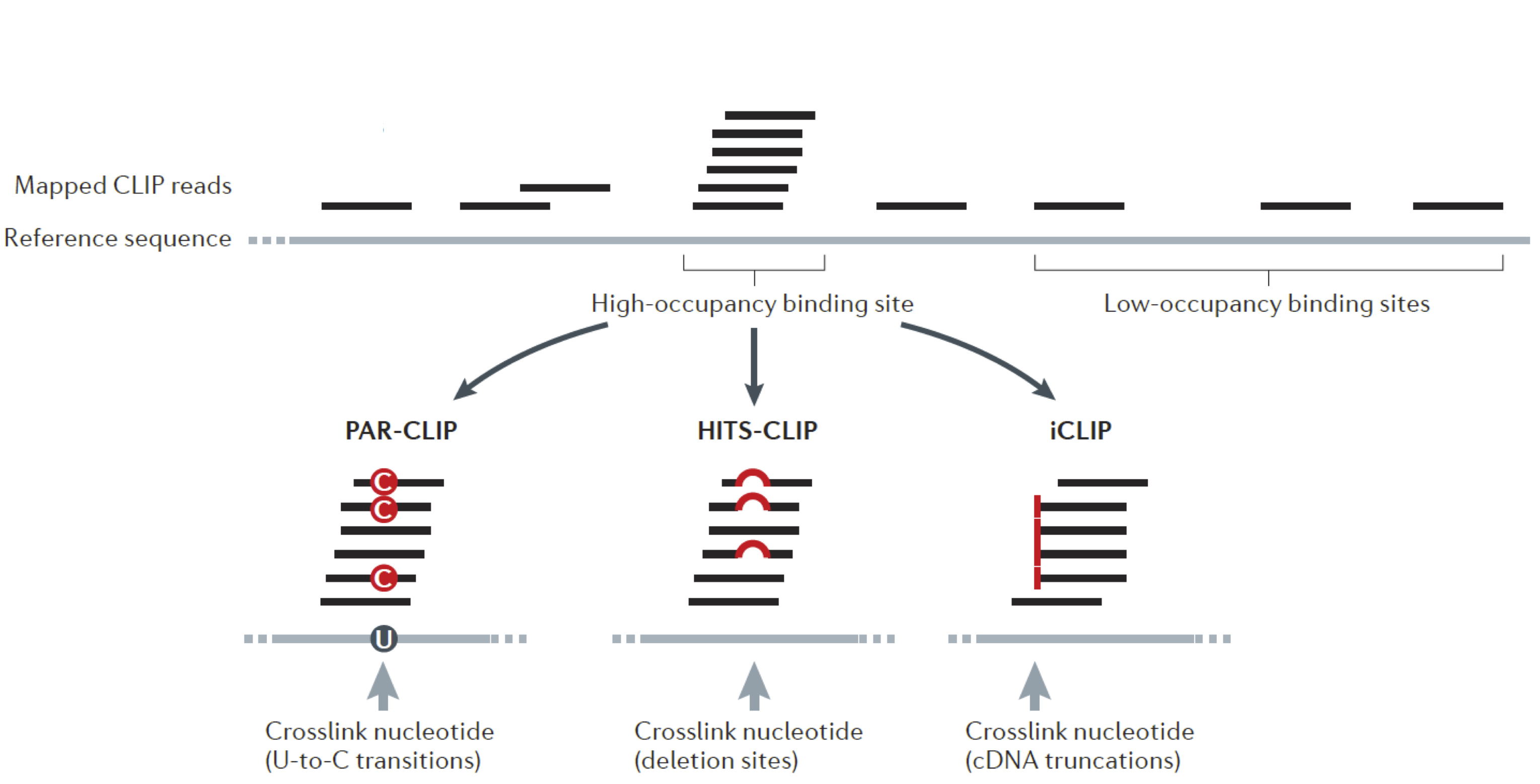
- T -> C transitions provide nucleotide resolution binding
- During cDNA generation, preferential base pairing of the 4SU crosslink product to a guanine instead of an adenine results in a thymine (T) to cytosine (C) transition in the PCR-amplified sequence, serving as a diagnostic mutation at the site of contact.
Mapping of RBP binding sites: analysis
Most CLIP-seq approaches have single-nucleotide resolution information. However, they vary in the frequency of that information and the efficiency of the procedure.
The basic concept to call a peak/binding sites from CLIP-seq:
- Map the reads to genome/transcriptome
- Group overlapping reads
- Use nucleotide level information to de/refine position of RBP-binding sites
In this class we will be working with PAR-CLIP data. Regardless, I will show you how to access ENCODE eCLIP data. You would easily be able to apply what you learn on those data.
Analysis overview
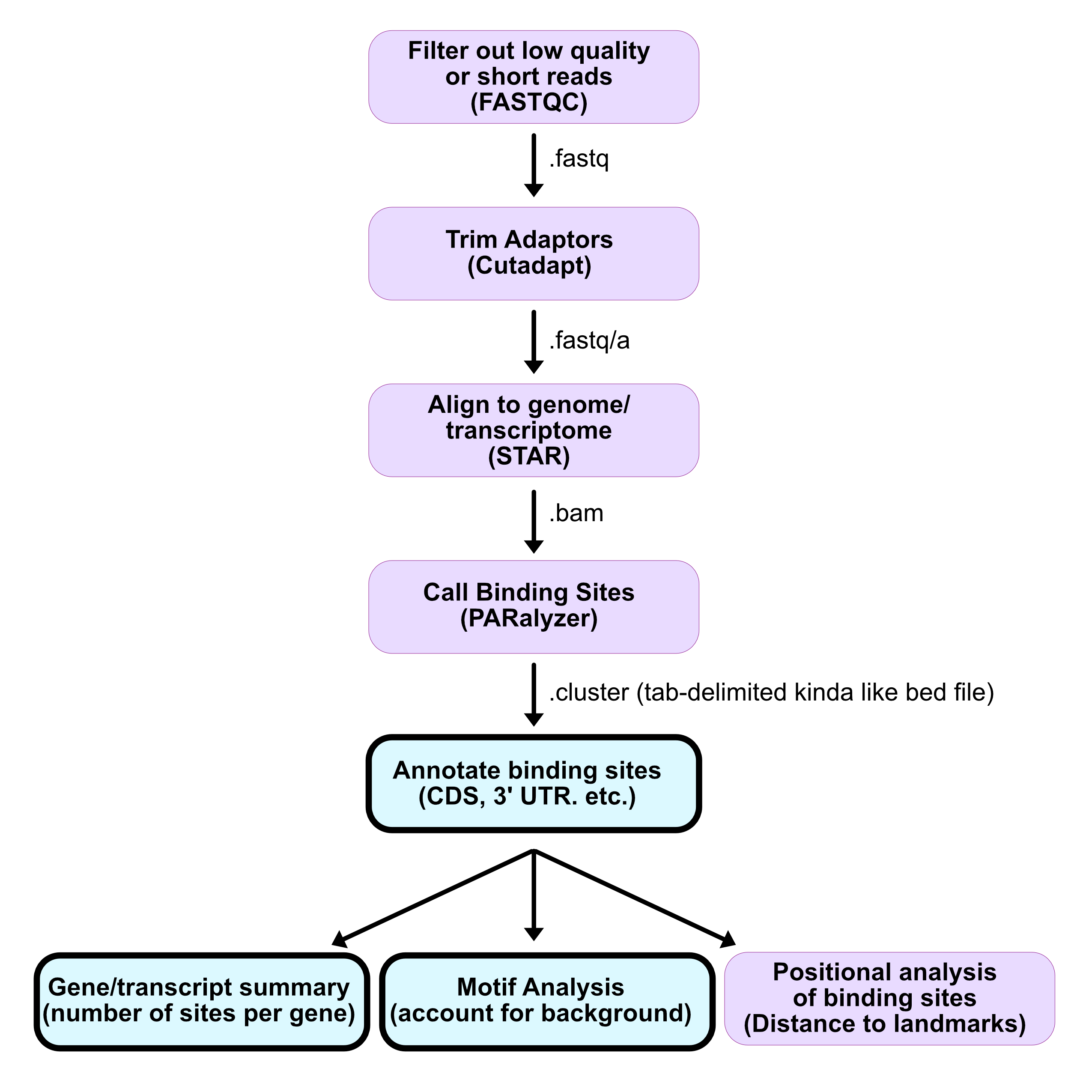
- Filter out low quality or short reads (<18 for larger genomes)
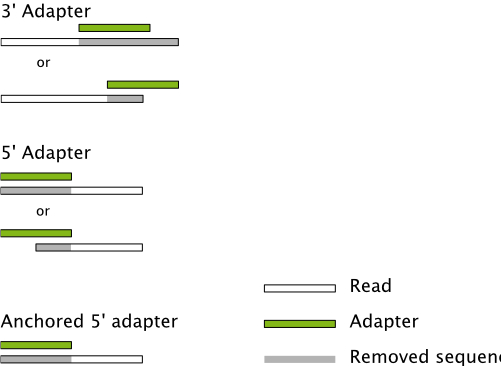
- Trim adapters
- Collapse PCR duplicate reads (molecular indexes)
- Align to genome/transcriptome
- Call peaks
- Downstream analysis
Pre-processing
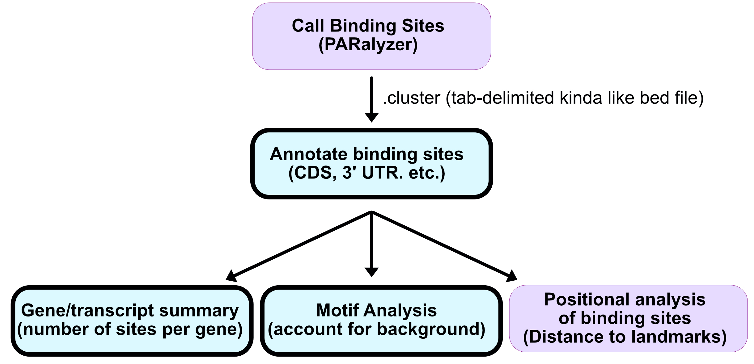
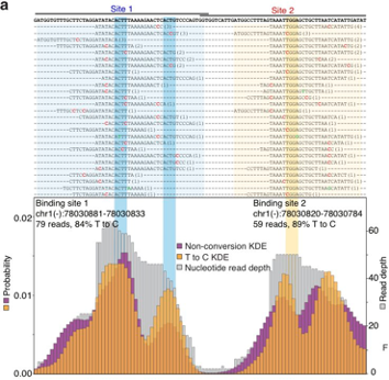
Calling binding sites: PARalyzer
The pattern of T = > C conversions, coupled with read density, can thus provide a strong signal to generate a high-resolution map of confident RNA-protein interaction sites.
A non-parametric kernel-density estimate used to identify the RNA-protein interaction sites from a combination of T = > C conversions and read density.
See PARalyzer for more information.
Annotation of binding sites
Where are the binding sites?
- Which genes?
- What region of those genes?
- How many binding sites per region?
- How many binding sites per gene?
- How many binding sites per gene by region?
We will use annotatr and Granges to answer these questions.

Set up annotation database
Extract annotation categories
What information is contained within the annotations object?
my_hg19_annots[3]

# get introns
annotation_introns <- annotations[annotations$type == ??]

# collapsing introns
annotation_introns <- GenomicRanges::reduce(annotation_introns)

# length of each intron interval
length_introns <- width(??)

#get cds
annotation_cds <- annotations[annotations$type == my_hg19_annots[1]]

# collapsing cds
annotation_cds <- GenomicRanges::reduce(annotation_cds)

# length of each cds interval
length_cds <- width(annotation_cds)
Compare introns and cds length
all_length <- bind_rows(
  tibble(nt=??,
       cat=rep("??",
               length(??))),

  tibble(nt=length_cds,
       cat=rep("cds",
               length(length_cds)))
)

ggplot(all_length,
       aes(x=??, color=??)) +
  geom_density() +
  scale_x_log10(breaks = trans_breaks("log10",
                                      function(x) 10^x),
                labels = trans_format("log10",
                                      math_format(10^.x))) +
  theme_cowplot()
The typical* human intron is way longer than a CDS exon.
ELAVL1/HuR
ELAVL1/HuR is an essential RNA-binding protein (RBP).
HuR binds to AU-rich elements (ARE) in 3’ UTRs of mRNAs to promote mRNA stability.
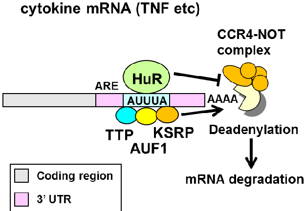
This model makes a few specific prediction:
- HuR binds to the 3’ UTR.
- HuR binds to AU-rich sequences (AUUUA).
- HuR binding promotes target RNA stabilization (and binding by the other RBPs to the ARE promotes destabilization).
We will explore these predictions during the next couple classes.
PAR-CLIP data
Reminder that we will be using this resource: rag-tag ENCODE
We are looking for an ELAVL1 PAR-CLIP corresponding to this SRA (short-read archive) ID: SRR248532
hur_regions <- read_regions(con = "https://raw.githubusercontent.com/BIMSBbioinfo/RCAS_meta-analysis/master/rbp-binding-sites/??.clusters.bed",
                            genome = 'hg19',
                            format = '??')


# looks like there are 111236 binding sites!!!
# we are only going to keep those w/a score > 1
# this will reduce it down to ~20K sites
# the score reflects the frequency of T->C conversions vs no conversion and non-T->C conversions per binding site
hur_regions <- hur_regions[hur_regions$score > 1]

hur_regions
Annotate PAR-CLIP data
# let's annotate
hur_annot <- annotate_regions(
    regions = ??,
    annotations = annotations,
    ignore.strand = FALSE,
    quiet = FALSE) %>%
  data.frame()


# we put in ~20K and got ~50K??

# redundant info due to transcript_id

# keep only columns we need
myInfo <- c("seqnames","start","end","width","strand","annot.symbol","annot.type")

hur_annot <- hur_annot[,??] %>%
  unique()

# getting rid of the "hg19_genes_" string to simplify `annot.type`
hur_annot$annot.type <- gsub("hg19_genes_","",hur_annot$annot.type)

table()
HuR binding region preference
It looks like HuR prefers binding to 3’ UTRs and introns. That is a bit of a surprise given the model above indicating 3’ UTR binding. Well let’s take a step back and frame our expectation using what we know about the genome.
For example, how much of the genome is coding?
In this case, how many basepairs are introns and 3’ UTRs in the genome?
binding region length biases
# total intron length
# sum(
#   width(
#     GenomicRanges::reduce(
#       annotations[annotations$type %in% my_hg19_annots[3]]
#       )
#     )
#   )

mylengths <- vector()

for (i in 1:length(my_hg19_annots)) {
  mylengths[i] <- sum(width(GenomicRanges::reduce(annotations[annotations$type %in% my_hg19_annots[i]])))

  names(mylengths)[i] <- gsub("hg19_genes_","",my_hg19_annots[i])


}

barplot(mylengths[1:4], las=2, main = "total bases per category", log="y")
Control for CLIP-binding sites
We need a way to figure out a null model OR background expectation.
What if we were to take our HuR binding and randomize their position and then repeat the annotation on the randomized binding sites?
# randomize regions based on par-clip regions
random_sites <- ??(
  regions = hur_regions,
  allow.overlaps = TRUE,
  per.chromosome = TRUE)

# annotate  randomize regions
random_sites_annot <- annotate_regions(
  regions = ??,
  annotations = annotations,
  ignore.strand = FALSE,
  quiet = FALSE) %>%
  data.frame()

# select cols, keep unique
random_sites_annot <- random_sites_annot[,myInfo] %>%
  unique()

# clean names
random_sites_annot$annot.type <- gsub("hg19_genes_","",random_sites_annot$annot.type)


table(random_sites_annot$annot.type)
Compare HuR vs Random
# create a new tibble with the annotation counts for hur (observed) and random (expected) binding sties
site_dist <- bind_cols(
  region=names(table(hur_annot$annot.type)),
  observed=table(??$annot.type),
  expected=table(??$annot.type)
          ) %>%
  mutate(enrichment = observed/expected) # calculate enrichment


site_dist_long <- pivot_longer(site_dist,
                               cols = c(??,??,??)
                               )

colnames(site_dist_long) <- c("region","type","value")

# plot counts for parclip vs random barplot
# ggplot(site_dist_long %>% filter(type!="enrichment"),
#        aes(y = value, x = region, fill = type)) +
#   geom_bar(stat="identity", position=position_dodge()) +
#   scale_fill_manual(values=c("black","red")) +
#   theme_cowplot()

# plot enrichment barplot
ggplot(site_dist_long %>% filter(type=="??"),
       aes(y = ??,
           x = ??)) +
  geom_bar(stat="identity") +
  ylab("Observed vs Expected") +
  theme_cowplot()
5 MINUTE BREAK
What sequence does HuR bind to?
Is it just AUUUA?
Different transcript regions have different nucleotide composition.
5’ UTRs are more GC-rich
3’ UTRs are more AU-rich
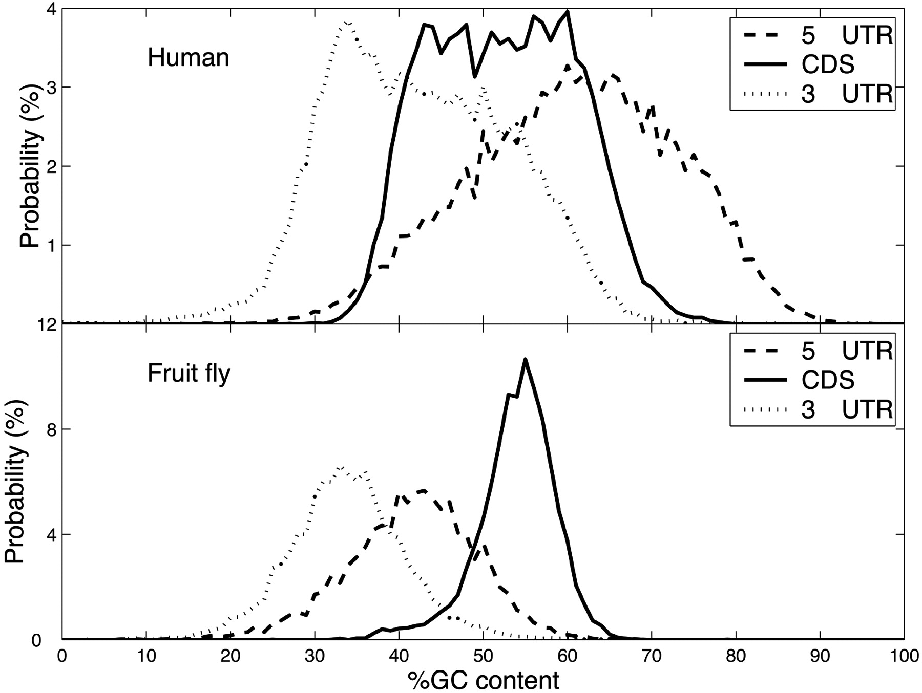
We need to account for these differences when asking what the binding preferences are for sites in a given transcript region.
Counting k-mers
Steps to determine k-mer composition (we use 6mers) for any set of intervals
We’ll do it for both HuR binding sites and then compare it to background seqs.
- Create a
Grangesobject for a given annotation category.
- Remove duplicated intervals (from diff transcript ids) with
reduce.
- Retrieve seqeunces using
getSeqs - Create a dataframe containing the count and frequency of each 6mer.
Calculate 6mers in HuR sites
Since HuR preferentially binds to 3’ UTRs, that is the region we will focus on.
# create a Grange for 3' UTRs
hur_3utr <- makeGRangesFromDataFrame(
  df = hur_annot %>% filter(??=="??"),
  ignore.strand = F,
  seqnames.field = "seqnames",
  start.field = "start",
  end.field = "end",
  strand.field = "strand",
  keep.extra.columns = T
  )

# get  sequencees for those coordinates
hur_3utr_seqs <- getSeq(BSgenome.Hsapiens.UCSC.hg19, ??)

# count  all 6 mer instances per sequence, add all instances, and turn into a dataframe with column name counts
hur_utr3_6mer <- ??(
  x = ??,
  width = 6, # k
  as.prob = F,
  simplify.as="matrix") %>%
  colSums() %>%
  as.data.frame()

colnames(hur_utr3_6mer) <- "hur_utr_count"

# calc freq
hur_utr3_6mer$hur_utr_freq <- hur_utr3_6mer$hur_utr_count/sum(hur_utr3_6mer$hur_utr_count)
Calculate 6mers in 3utrs
Next, we will calculate 6mer frequencies in 3’ UTRs. This will serve as a null model or background that we can compare with the HuR binding site 6mers.
# create a Grange for 3' UTRs
threeUTR <- GenomicRanges::reduce(annotations[annotations$type %in% my_hg19_annots[??]])

# get sequences for those coordinates
threeUTR_seqs <- getSeq(BSgenome.Hsapiens.UCSC.hg19, threeUTR)

# count  all 6 mer instances per sequence, add all instances, and turn into a dataframe with column name counts
utr3_6mer <- ??(
  x = ??,
  width = 6,
  as.prob = F,
  simplify.as="matrix") %>%
  colSums() %>%
  as.data.frame()

colnames(utr3_6mer) <- "utr_count"

# calc freq
utr3_6mer$utr_freq <- utr3_6mer$utr_count/sum(utr3_6mer$utr_count)
Sequences enriched in hur sites vs 3utr
# check if rownames are identical and stop if they are  not
stopifnot(identical(rownames(hur_utr3_6mer),rownames(utr3_6mer)))

# bind_cols
utr3_df <- bind_cols(hur_utr3_6mer,
                     utr3_6mer)
# Calc enrichment
utr3_df$hur_enrich <- utr3_df$hur_utr_freq/utr3_df$utr_freq


# plot coloring and labeling all > 8 fold enriched
ggplot(data = utr3_df,
       aes(y = ??, # hur
           x = ?? # utrs
             )
       ) +
  geom_point(color = ifelse(utr3_df$hur_enrich > 8, "red", "black")) +
  ylab("kmers: HuR 3'UTR sites") +
  xlab("kmers: 3'UTR") +
  geom_abline(intercept = 0, slope = 1) +
  geom_text_repel(aes(label=ifelse(hur_enrich > 8,
                                   rownames(utr3_df),
                                   ""))) +
  theme_cowplot()
Sequences enriched in hur sites vs 3utr
Not just AU-rich…
utr3_df %>%
  rownames_to_column(var = "6mer") %>%
  arrange(-hur_enrich) %>%
  gt()