Interval statistics

Overview

valr includes several functions for exploring statistical relationships between sets of intervals.

Calculate significance of overlaps between sets of intervals with bed_fisher() and bed_projection().
Quantify relative and absolute distances between sets of intervals with bed_reldist() and bed_absdist().
Quantify extent of overlap between sets of intervals with bed_jaccard().

In this vignette we explore the relationship between transcription start sites and repetitive elements in the human genome.

library(valr)
library(dplyr)
library(ggplot2)
library(cowplot)
library(tidyr)

# load repeats and genes. Data in the valr package is restricted to chr22; the entire
# files can be downloaded from UCSC.
rpts <- read_bed(valr_example("hg19.rmsk.chr22.bed.gz"))
genes <- read_bed12(valr_example("hg19.refGene.chr22.bed.gz"))

# load chrom sizes
genome <- read_genome(valr_example("hg19.chrom.sizes.gz"))

# create 1 bp intervals representing transcription start sites
tss <- create_tss(genes)

tss
#> # A tibble: 1,267 × 6
#>    chrom    start      end name         score strand
#>    <chr>    <dbl>    <dbl> <chr>        <chr> <chr> 
#>  1 chr22 16193008 16193009 NR_122113    0     -     
#>  2 chr22 16157078 16157079 NR_133911    0     +     
#>  3 chr22 16162065 16162066 NR_073459    0     +     
#>  4 chr22 16162065 16162066 NR_073460    0     +     
#>  5 chr22 16231288 16231289 NR_132385    0     -     
#>  6 chr22 16287936 16287937 NM_001136213 0     -     
#>  7 chr22 16274608 16274609 NR_046571    0     +     
#>  8 chr22 16449803 16449804 NM_001005239 0     -     
#>  9 chr22 17073699 17073700 NM_014406    0     -     
#> 10 chr22 17082800 17082801 NR_001591    0     +     
#> # ℹ 1,257 more rows

Distance metrics

First we define a function that takes x and y intervals and computes distance statistics (using bed_reldist() and bed_absdist()) for specified groups. The value of each statistic is assigned to a .value column.

distance_stats <- function(x, y, genome, group_var, type = NA) {
  group_by(x, !!rlang::sym(group_var)) |>
    do(
      reldist = bed_reldist(., y, detail = TRUE) |>
        select(.value = .reldist),
      absdist = bed_absdist(., y, genome) |>
        select(.value = .absdist)
    ) |>
    tidyr::pivot_longer(
      cols = -name,
      names_to = "stat",
      values_to = "value"
    ) |>
    mutate(type = type)
}

We use the distance_stats() function to apply the bed_absdist() function to each group of data.

obs_stats <- distance_stats(rpts, tss, genome, "name", "obs")
obs_stats
#> # A tibble: 2,106 × 4
#>    name       stat    value             type 
#>    <chr>      <chr>   <list>            <chr>
#>  1 (A)n       reldist <tibble [27 × 1]> obs  
#>  2 (A)n       absdist <tibble [28 × 1]> obs  
#>  3 (AAAAACA)n reldist <tibble [1 × 1]>  obs  
#>  4 (AAAAACA)n absdist <tibble [1 × 1]>  obs  
#>  5 (AAAAC)n   reldist <tibble [6 × 1]>  obs  
#>  6 (AAAAC)n   absdist <tibble [7 × 1]>  obs  
#>  7 (AAAAG)n   reldist <tibble [2 × 1]>  obs  
#>  8 (AAAAG)n   absdist <tibble [2 × 1]>  obs  
#>  9 (AAAAT)n   reldist <tibble [3 × 1]>  obs  
#> 10 (AAAAT)n   absdist <tibble [4 × 1]>  obs  
#> # ℹ 2,096 more rows

And the same is done for a set of shuffled group of data. bed_shuffle() is used to shuffle coordinates of the repeats within each chromosome (i.e., the coordinates change, but the chromosome stays the same.)

shfs <- bed_shuffle(rpts, genome, within = TRUE)
shf_stats <- distance_stats(shfs, tss, genome, "name", "shuf")

Now we can bind the observed and shuffled data together, and do some tidying to put the data into a format appropriate for a statistical test. This involves:

unnest()ing the data frames
creating groups for each repeat (name), stat (reldist or absdist) and type (obs or shf)
adding unique surrogate row numbers for each group
using tidyr::pivot_wider() to create two new obs and shuf columns
removing rows with NA values.

res <- bind_rows(obs_stats, shf_stats) |>
  tidyr::unnest(value) |>
  group_by(name, stat, type) |>
  mutate(.id = row_number()) |>
  tidyr::pivot_wider(
    names_from = "type",
    values_from = ".value"
  ) |>
  na.omit()

res
#> # A tibble: 16,785 × 5
#> # Groups:   name, stat [1,904]
#>    name  stat      .id   obs  shuf
#>    <chr> <chr>   <int> <dbl> <dbl>
#>  1 (A)n  reldist     1 0.363 0.177
#>  2 (A)n  reldist     2 0.429 0.404
#>  3 (A)n  reldist     3 0.246 0.119
#>  4 (A)n  reldist     4 0.478 0.157
#>  5 (A)n  reldist     5 0.260 0.176
#>  6 (A)n  reldist     6 0.286 0.225
#>  7 (A)n  reldist     7 0.498 0.128
#>  8 (A)n  reldist     8 0.237 0.385
#>  9 (A)n  reldist     9 0.314 0.413
#> 10 (A)n  reldist    10 0.149 0.234
#> # ℹ 16,775 more rows

Now that the data are formatted, we can use the non-parametric ks.test() to determine whether there are significant differences between the observed and shuffled data for each group. broom::tidy() is used to reformat the results of each test into a tibble, and the results of each test are pivoted to into a type column for each test type.

library(broom)

pvals <- res |>
  do(
    twosided = tidy(ks.test(.$obs, .$shuf)),
    less = tidy(ks.test(.$obs, .$shuf, alternative = "less")),
    greater = tidy(ks.test(.$obs, .$shuf, alternative = "greater"))
  ) |>
  tidyr::pivot_longer(cols = -c(name, stat), names_to = "alt", values_to = "type") |>
  unnest(type) |>
  select(name:p.value) |>
  arrange(p.value)

Histgrams of the different stats help visualize the distribution of p.values.

ggplot(pvals, aes(p.value)) +
  geom_histogram(binwidth = 0.05) +
  facet_grid(stat ~ alt) +
  theme_cowplot()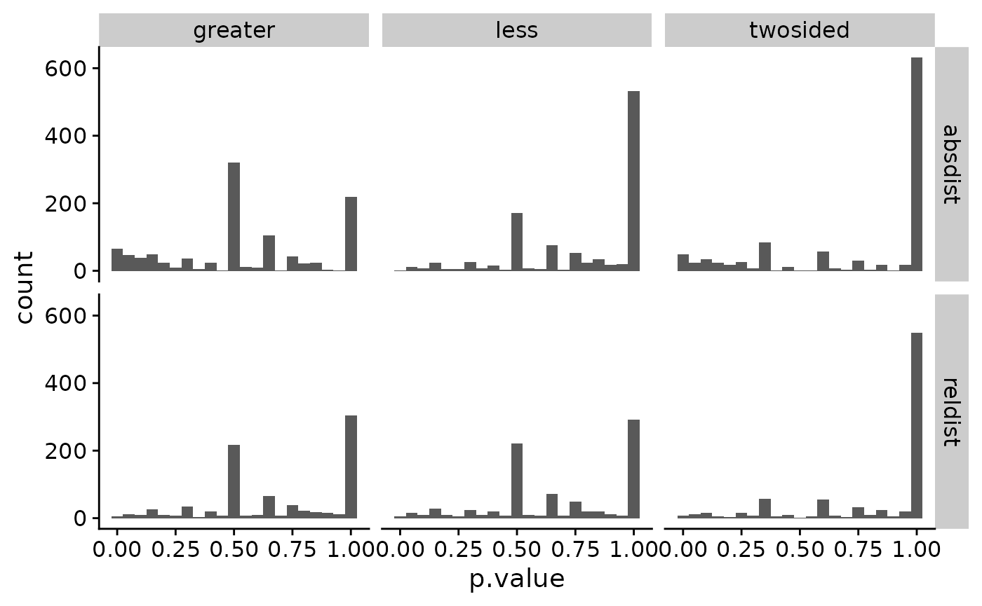

We can also assess false discovery rates (q.values) using p.adjust().

pvals <-
  group_by(pvals, stat, alt) |>
  mutate(q.value = p.adjust(p.value)) |>
  ungroup() |>
  arrange(q.value)

Finally we can visualize these results using stat_ecdf().

res_gather <- tidyr::pivot_longer(res,
  cols = -c(name, stat, .id),
  names_to = "type",
  values_to = "value"
)

signif <- head(pvals, 5)

res_signif <-
  signif |>
  left_join(res_gather, by = c("name", "stat"))
#> Warning in left_join(signif, res_gather, by = c("name", "stat")): Detected an unexpected many-to-many relationship between `x` and `y`.
#> ℹ Row 1 of `x` matches multiple rows in `y`.
#> ℹ Row 29037 of `y` matches multiple rows in `x`.
#> ℹ If a many-to-many relationship is expected, set `relationship =
#>   "many-to-many"` to silence this warning.

ggplot(res_signif, aes(x = value, color = type)) +
  stat_ecdf() +
  facet_grid(stat ~ name) +
  theme_cowplot() +
  scale_x_log10() +
  scale_color_brewer(palette = "Set1")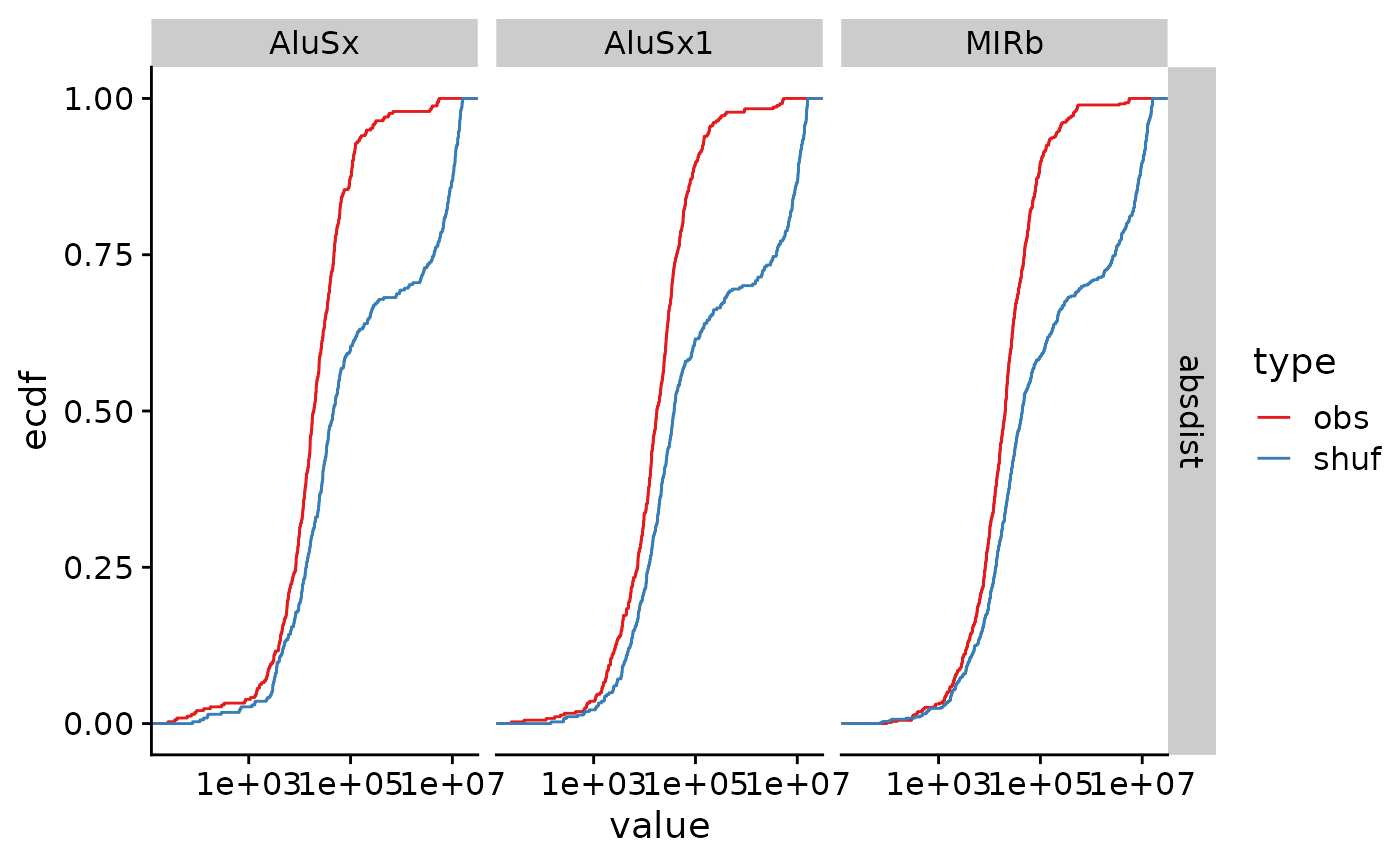

Projection test

bed_projection() is a statistical approach to assess the relationship between two intervals based on the binomial distribution. Here, we examine the distribution of repetitive elements within the promoters of coding or non-coding genes.

First we’ll extract 5 kb regions upstream of the transcription start sites to represent the promoter regions for coding and non-coding genes.

# create intervals 5kb upstream of tss representing promoters
promoters <-
  bed_flank(genes, genome, left = 5000, strand = TRUE) |>
  mutate(name = ifelse(grepl("NR_", name), "non-coding", "coding")) |>
  select(chrom:strand)

# select coding and non-coding promoters
promoters_coding <- filter(promoters, name == "coding")
promoters_ncoding <- filter(promoters, name == "non-coding")

promoters_coding
#> # A tibble: 973 × 6
#>    chrom    start      end name   score strand
#>    <chr>    <int>    <int> <chr>  <chr> <chr> 
#>  1 chr22 16287937 16292937 coding 0     -     
#>  2 chr22 16449804 16454804 coding 0     -     
#>  3 chr22 17073700 17078700 coding 0     -     
#>  4 chr22 17302589 17307589 coding 0     -     
#>  5 chr22 17302589 17307589 coding 0     -     
#>  6 chr22 17489112 17494112 coding 0     -     
#>  7 chr22 17560848 17565848 coding 0     +     
#>  8 chr22 17560848 17565848 coding 0     +     
#>  9 chr22 17602213 17607213 coding 0     -     
#> 10 chr22 17602257 17607257 coding 0     -     
#> # ℹ 963 more rows

promoters_ncoding
#> # A tibble: 294 × 6
#>    chrom    start      end name       score strand
#>    <chr>    <int>    <int> <chr>      <chr> <chr> 
#>  1 chr22 16152078 16157078 non-coding 0     +     
#>  2 chr22 16157065 16162065 non-coding 0     +     
#>  3 chr22 16157065 16162065 non-coding 0     +     
#>  4 chr22 16193009 16198009 non-coding 0     -     
#>  5 chr22 16231289 16236289 non-coding 0     -     
#>  6 chr22 16269608 16274608 non-coding 0     +     
#>  7 chr22 17077800 17082800 non-coding 0     +     
#>  8 chr22 17156430 17161430 non-coding 0     -     
#>  9 chr22 17229328 17234328 non-coding 0     -     
#> 10 chr22 17303363 17308363 non-coding 0     +     
#> # ℹ 284 more rows

Next we’ll apply the bed_projection() test for each repeat class for both coding and non-coding regions.

# function to apply bed_projection to groups
projection_stats <- function(x, y, genome, group_var, type = NA) {
  group_by(x, !!rlang::sym(group_var)) |>
    do(
      n_repeats = nrow(.),
      projection = bed_projection(., y, genome)
    ) |>
    mutate(type = type)
}

pvals_coding <- projection_stats(rpts, promoters_coding, genome, "name", "coding")
pvals_ncoding <- projection_stats(rpts, promoters_ncoding, genome, "name", "non_coding")

pvals <-
  bind_rows(pvals_ncoding, pvals_coding) |>
  ungroup() |>
  tidyr::unnest(cols = c(n_repeats, projection)) |>
  select(-chrom)

# filter for repeat classes with at least 10 intervals
pvals <- filter(
  pvals,
  n_repeats > 10,
  obs_exp_ratio != 0
)

# adjust pvalues
pvals <- mutate(pvals, q.value = p.adjust(p.value))

pvals
#> # A tibble: 179 × 7
#>    name   n_repeats p.value obs_exp_ratio lower_tail type       q.value
#>    <chr>      <int>   <dbl>         <dbl> <chr>      <chr>        <dbl>
#>  1 (A)n          28 0.00353         4.72  FALSE      non_coding   0.558
#>  2 (AT)n         48 0.298           0.917 FALSE      non_coding   1    
#>  3 (CA)n         31 0.156           1.42  FALSE      non_coding   1    
#>  4 (GT)n         42 0.247           1.05  FALSE      non_coding   1    
#>  5 (T)n          61 0.405           0.721 FALSE      non_coding   1    
#>  6 (TG)n         40 0.0622          2.20  FALSE      non_coding   1    
#>  7 A-rich        54 0.348           0.815 FALSE      non_coding   1    
#>  8 Alu           15 0.0446          2.93  FALSE      non_coding   1    
#>  9 AluJb        271 0.0225          1.79  FALSE      non_coding   1    
#> 10 AluJo        208 0.0216          1.90  FALSE      non_coding   1    
#> # ℹ 169 more rows

The projection test is a two-tailed statistical test. A significant p-value indicates either enrichment or depletion of query intervals compared to the reference interval sets. A value of lower_tail = TRUE column indicates that the query intervals are depleted, whereas lower_tail = FALSE indicates that the query intervals are enriched.

library(DT)

# find and show top 5 most significant repeats
signif_tests <-
  pvals |>
  arrange(q.value) |>
  group_by(type) |>
  top_n(-5, q.value) |>
  arrange(type)

DT::datatable(signif_tests)

June 22 2025

Overview

Distance metrics

Projection test